
Energy Beyond Particle Mechanics
Physics ·This note continues Rediscovering Mechanics and Energy from Questions, which introduced kinetic and potential energy using a cart attached to a spring. That construction leaves one main question:
Are kinetic and potential energy the only possible kinds of energy, or are they merely the parts that happened to be useful for that problem?
We will follow the same method as before: begin with a question, use the measured update rules to answer it, and introduce a new energy term only when the calculation requires one.
1. What did energy accomplish for one cart?
For the cart and spring, the original question was to predict quantities such as the cart’s maximum speed without calculating every intermediate position. The update rules led to two endpoint quantities:
\[K(v)=\frac12mv^2, \qquad U(x)=\frac12kx^2.\]The spring’s work increased one by exactly the amount that it decreased the other:
\[\Delta K=-\Delta U.\]Therefore,
\[E=K+U\]remained constant, allowing us to compare the initial and final states directly.
That was the role of energy: it compressed many moment-by-moment updates into a relation between states. Calling the two terms kinetic and potential energy did not establish that nature contains exactly two fundamental substances. It identified two quantities that were convenient—and, given the measured dynamics, mathematically effective—for answering the question.
Does the same construction appear without a moving mass?
Consider an ideal electrical circuit containing an inductor and a capacitor. Let \(Q(t)\) be the capacitor’s charge and let
\[I=\frac{dQ}{dt}\]be the current. The circuit’s update rule is
\[L\frac{dI}{dt}=-\frac{Q}{C},\]where \(L\) is the inductance and \(C\) is the capacitance.
Ask the same kind of question as before:
Can we construct an endpoint quantity that remains constant and lets us relate the circuit’s present and future states?
The update rules give
\[\begin{aligned} \frac{d}{dt}\left(\frac12LI^2+\frac12\frac{Q^2}{C}\right) &=LI\frac{dI}{dt}+\frac{Q}{C}\frac{dQ}{dt}\\ &=I\left(L\frac{dI}{dt}+\frac{Q}{C}\right)\\ &=0. \end{aligned}\]Therefore the circuit has the conserved quantity
\[E=\frac12LI^2+\frac12\frac{Q^2}{C}.\]It has exactly the same mathematical pattern as the cart-spring energy:
\[E=\frac12mv^2+\frac12kx^2.\]| Mechanical system | Electrical circuit |
|---|---|
| Position \(x\) | Charge \(Q\) |
| Velocity \(v\) | Current \(I\) |
| Mass \(m\) | Inductance \(L\) |
| Spring stiffness \(k\) | Inverse capacitance \(1/C\) |
| Kinetic energy | Magnetic energy of the inductor |
| Spring potential energy | Electric energy of the capacitor |
The circuit contains no cart whose position is \(Q\) and no mechanical mass equal to \(L\). The analogy shows that the two-part structure can arise from the form of the update rules, while the physical interpretation of its terms changes with the system.
The new problem is to determine what happens when the state of a system requires more than one changing value.
2. What is a degree of freedom?
A degree of freedom is one independent value needed to specify a configuration.
| System | Values needed to specify its configuration |
|---|---|
| One cart on a line | One position \(x\) |
| Two carts on a line | Two positions \(x_1,x_2\) |
| \(N\) movable points | \(N\) positions \(x_1,\ldots,x_N\) |
| A field | One value at every point in space |
For a particle, the configuration at time \(t\) is specified by finitely many coordinates, such as \(x(t)\). For a field, the configuration at time \(t\) is an entire function \(\phi(\mathbf{x},t)\). Thus a field has effectively one degree of freedom at every point in space.
This definition raises a concrete question:
If different degrees of freedom affect one another, what endpoint quantity lets us predict their possible later states without solving every intermediate update?
We can answer it first for only two degrees of freedom.
3. Why does a coupling term appear?
Consider two equal carts, each with mass \(m\), connected by a spring with stiffness \(k\). Let \(x_1(t)\) and \(x_2(t)\) be their displacements from equilibrium. The spring’s change in extension is then \(x_1-x_2\). Suppose experiments give the update rules
\[\begin{aligned} m\ddot x_1&=-k(x_1-x_2),\\ m\ddot x_2&=\phantom{-}k(x_1-x_2). \end{aligned}\]We ask:
Given the present positions and velocities, can we construct a state quantity that remains fixed and therefore constrains the carts’ later velocities?
We do not need a new method. From the one-cart problem, the change in kinetic energy equals the work done. For both carts together, define
\[K=\frac12m\dot x_1^2+\frac12m\dot x_2^2.\]The total work done by the connecting spring from time \(t_1\) to \(t_2\) is the sum of the work done on the two carts:
\[\begin{aligned} W &=\int_{t_1}^{t_2} \left(F_1\dot x_1+F_2\dot x_2\right)dt\\ &=\int_{t_1}^{t_2} \left[-kr\dot x_1+kr\dot x_2\right]dt, \end{aligned}\]where
\[r:=x_1-x_2.\]Because \(\dot r=\dot x_1-\dot x_2\), the integral becomes
\[\begin{aligned} W &=-\int_{t_1}^{t_2}kr\dot r\,dt\\ &=-\int_{r_1}^{r_2}kr\,dr\\ &=-\left(\frac12kr_2^2-\frac12kr_1^2\right). \end{aligned}\]Thus the spring’s work depends only on the initial and final separations. Following the same endpoint construction as for the one-cart spring, define
\[U_{\mathrm{spring}}(x_1,x_2) :=\frac12kr^2 =\frac12k(x_1-x_2)^2.\]The work relation is therefore
\[W=-\Delta U_{\mathrm{spring}}.\]But the work-energy relation also gives
\[\Delta K=W.\]Combining them yields
\[\Delta K=-\Delta U_{\mathrm{spring}}, \qquad \Delta\left(K+U_{\mathrm{spring}}\right)=0.\]The coupling term is potential energy: it is the stored energy of the connecting spring. The word “coupling” does not name a third kind of energy. It says that this potential depends on a relationship between two degrees of freedom, \(x_1-x_2\), rather than on either position alone. The term arose because the measured update of \(x_1\) depended on \(x_2\) and vice versa.
4. Why does a field have spatial-gradient energy?
Begin with the spring force already developed in Section 3. Fix two identical springs to opposite walls and attach both to one mass. Let each wall be a horizontal distance \(a\) from the mass’s equilibrium position, and let each spring’s natural length be \(\ell_0<a\).
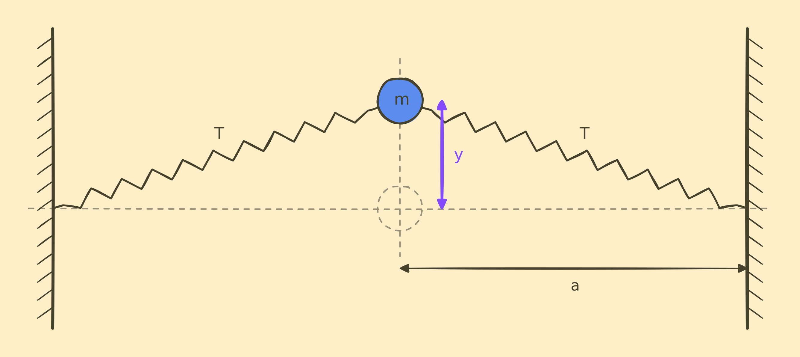
At \(y=0\), each spring pulls with magnitude
\[F_{\mathrm{s}}=k(a-\ell_0).\]The left and right forces point in opposite directions, so they cancel. Give this already-familiar spring force a shorter name:
\[T:=k(a-\ell_0).\]This is tension. It is not a new kind of force; it is the pulling force already carried by each stretched spring.
Now move the mass vertically by \(y\). Each spring has length
\[\ell(y)=\sqrt{a^2+y^2}\]and pulls with magnitude
\[F_{\mathrm{s}}(y)=k\bigl(\ell(y)-\ell_0\bigr).\]Here \(F_{\mathrm{s}}\) is the magnitude of the entire spring force, not its horizontal component. Put the displaced mass at \((0,y)\) and the two anchors at \((-a,0)\) and \((a,0)\). The vectors from the mass toward the anchors are
\[\mathbf r_{\mathrm{L}}=(-a,-y), \qquad \mathbf r_{\mathrm{R}}=(a,-y).\]Both have length \(\ell(y)\), so their unit directions are \(\mathbf r_{\mathrm{L}}/\ell(y)\) and \(\mathbf r_{\mathrm{R}}/\ell(y)\). Because each spring pulls along its own length, the two force vectors are
\[\begin{aligned} \mathbf F_{\mathrm{L}} &=\frac{F_{\mathrm{s}}(y)}{\ell(y)}(-a,-y),\\ \mathbf F_{\mathrm{R}} &=\frac{F_{\mathrm{s}}(y)}{\ell(y)}(a,-y). \end{aligned}\]Adding them gives
\[\begin{aligned} \mathbf F_{\mathrm{L}}+\mathbf F_{\mathrm{R}} &=\frac{F_{\mathrm{s}}(y)}{\ell(y)} \left[(-a,-y)+(a,-y)\right]\\ &=\left(0,-2F_{\mathrm{s}}(y)\frac{y}{\ell(y)}\right). \end{aligned}\]Thus the horizontal components cancel, while the vertical components add:
\[F_y =-2F_{\mathrm{s}}(y)\frac{y}{\ell(y)}.\]The magnitude law \(F_{\mathrm{s}}=k(\ell-\ell_0)\) and the fact that a spring pulls along its length belong to the measured spring model. Obtaining the horizontal and vertical components from that force is geometry.
For \(\lvert y\rvert\ll a\), we have \(F_{\mathrm{s}}(y)\approx T\) and \(\ell(y)\approx a\), so
\[F_y\approx-\frac{2T}{a}y.\]Thus tension is useful because the geometry converts two familiar spring forces into a restoring force for transverse motion.
How can the disturbance travel?
One mass can oscillate, but there is nowhere for a disturbance to travel. Now place finitely many masses in a row and join adjacent masses by spring segments that are already stretched and carry the same force \(T\). Hold the two ends fixed. Let \(\phi_i(t)\) be the vertical displacement of mass \(i\), and let neighboring equilibrium positions be separated by \(a\).
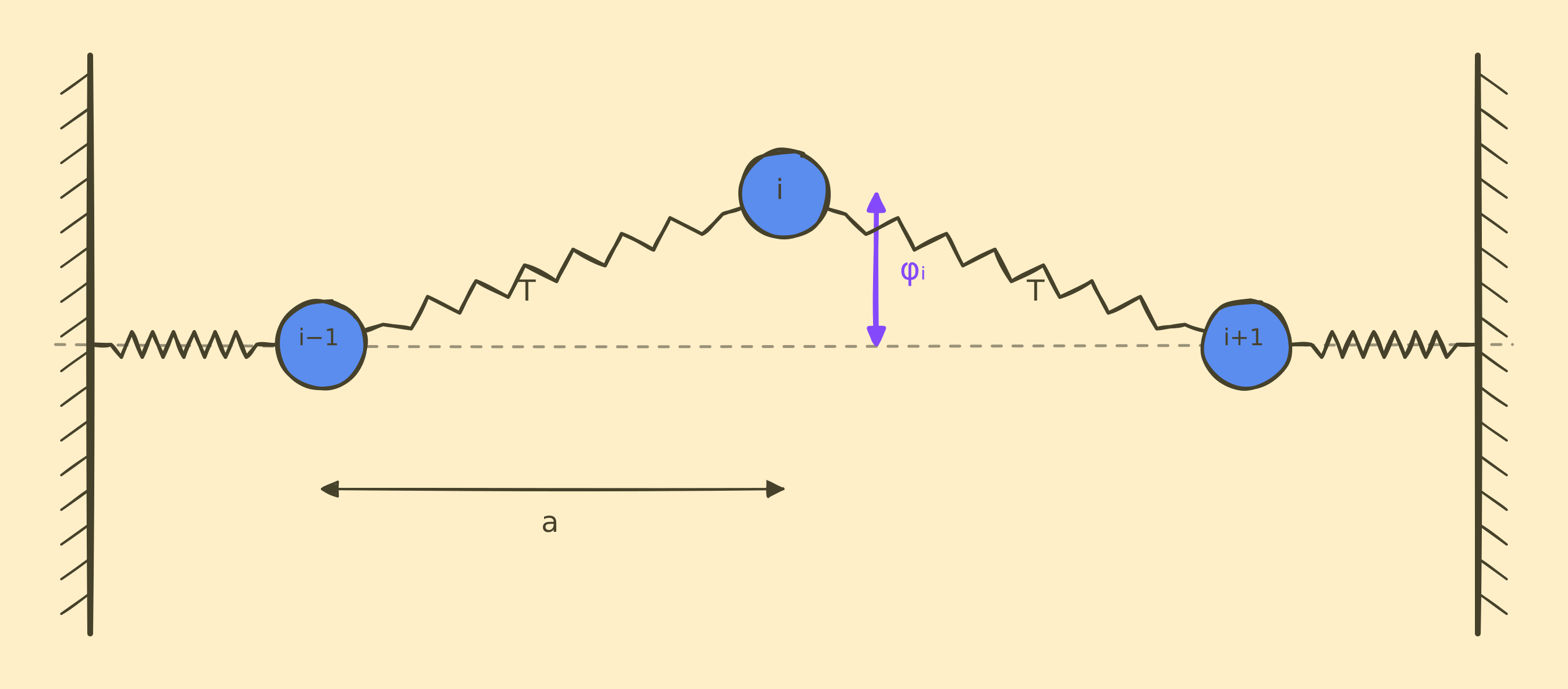
For small displacements, the right segment contributes the vertical force
\[T\frac{\phi_{i+1}-\phi_i}{a},\]while the left segment contributes
\[T\frac{\phi_{i-1}-\phi_i}{a}.\]Adding them gives the update equation
\[m\ddot\phi_i =\frac{T}{a} \left(\phi_{i+1}-2\phi_i+\phi_{i-1}\right).\]This answers the propagation question: changing \(\phi_i\) changes the forces on its neighbors, which then change their neighbors.
The segment joining sites \(i\) and \(i+1\) has length
\[\ell_i =\sqrt{a^2+(\phi_{i+1}-\phi_i)^2}.\]For \(\lvert\phi_{i+1}-\phi_i\rvert\ll a\), its increase in length is approximately
\[\Delta\ell_i \approx\frac{(\phi_{i+1}-\phi_i)^2}{2a}.\]Increasing a segment already carrying force \(T\) by this amount requires the work
\[U_i \approx T\Delta\ell_i =\frac{T}{2a}(\phi_{i+1}-\phi_i)^2.\]The finite chain therefore has the approximate energy
\[E_N =\sum_i\left[ \frac12m\dot\phi_i^2 +\frac{T}{2a}(\phi_{i+1}-\phi_i)^2 \right].\]Why introduce a field?
A guitar string is a continuous elastic object rather than a literal collection of carts. The finite chain tells us what information matters, but using one coordinate for every microscopic piece would be impractical. At scales much larger than the atomic spacing, define
\[\phi(x,t) :=\text{vertical displacement of the string at position }x\text{ and time }t.\]This is a field: at each time, its state is an entire function of position.
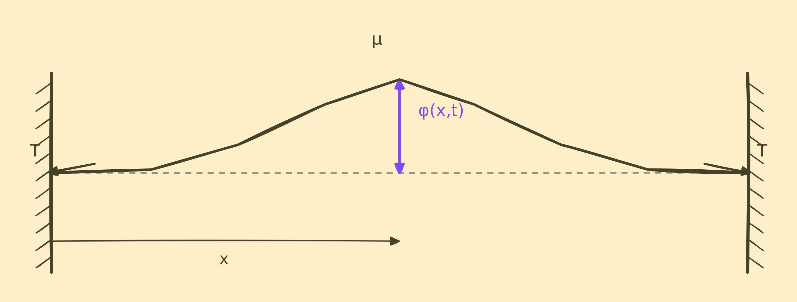
Divide the string into finite segments of length \(\Delta x\) and set \(m=\mu\Delta x\). The finite-chain energy becomes
\[E_N =\sum_i\left[ \frac12\mu\dot\phi_i^2 +\frac12T \left(\frac{\phi_{i+1}-\phi_i}{\Delta x}\right)^2 \right]\Delta x.\]As the largest segment length tends to zero, the finite differences approach the spatial derivative and this Riemann sum approaches
\[E =\int\left[ \frac12\mu\left(\frac{\partial\phi}{\partial t}\right)^2 +\frac12T\left(\frac{\partial\phi}{\partial x}\right)^2 \right]dx.\]The first term is kinetic energy distributed along the string. The second is potential energy: a bent string is longer than a straight one, so tension stores additional energy. Its update equation is the wave equation
\[\mu\frac{\partial^2\phi}{\partial t^2} =T\frac{\partial^2\phi}{\partial x^2}.\]The spatial-gradient term is therefore not a third fundamental kind of energy. It is the potential energy required by a real question about a continuous object: predicting how a plucked string moves.
Does a real system ever need a local term?
The guitar string does not need one. Its tension responds to differences between nearby displacements. To motivate a local term, we need a different physical question:
Can each degree of freedom be pulled toward equilibrium even when it agrees with all its neighbors?
Consider a row of identical pendulums whose neighboring bobs are connected by light springs:
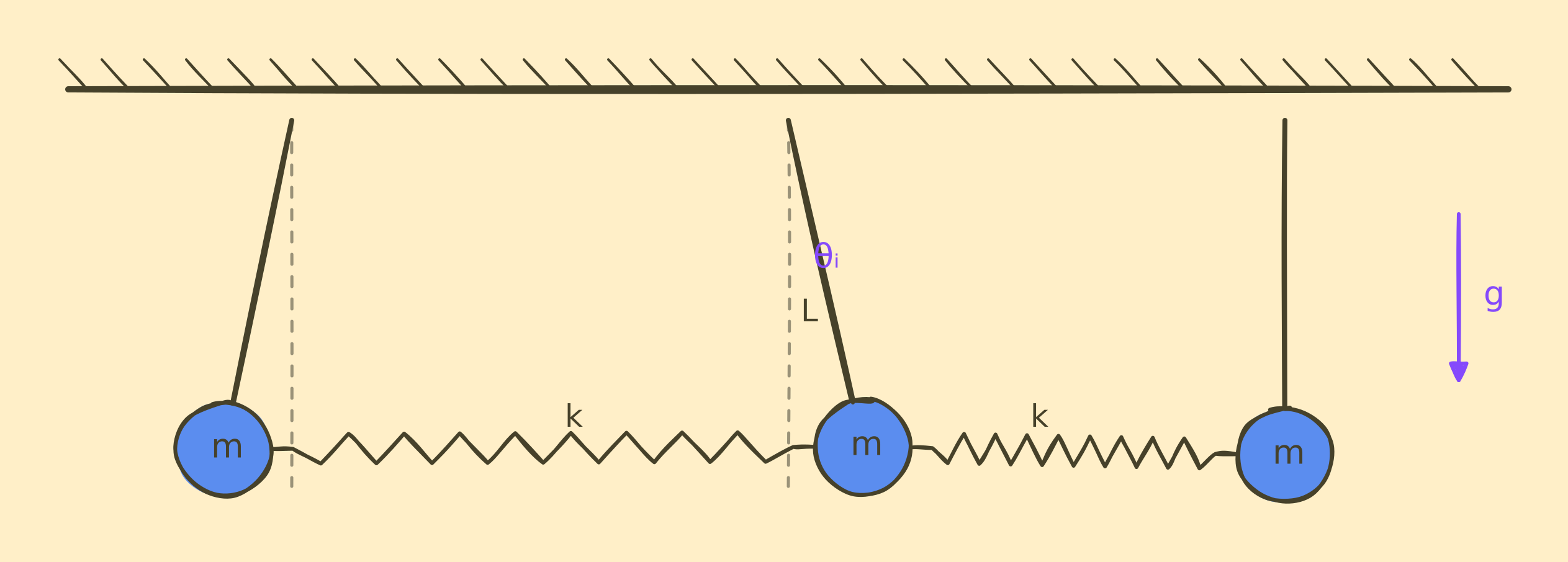
For pendulum \(i\), gravity gives the exact potential energy
\[V(\theta_i) =mgL(1-\cos\theta_i).\]This is local because it depends on \(\theta_i\) alone. For small angles,
\[V(\theta_i) \approx\frac12mgL\theta_i^2.\]The spring between neighboring bobs responds to their relative horizontal displacement. For small angles that displacement is approximately \(L(\theta_i-\theta_j)\), so its potential has the form
\[U(\theta_i-\theta_j) :=\frac12\kappa(\theta_i-\theta_j)^2,\]where \(\kappa\) includes the spring stiffness and the factor of \(L^2\). The approximate total energy is therefore
\[E =\sum_i\frac12mL^2\dot\theta_i^2 +\sum_{\langle i,j\rangle}U(\theta_i-\theta_j) +\sum_iV(\theta_i).\]Let \(U_{\mathrm{total}}\) denote both potential-energy sums. Only two neighbor terms contain \(\theta_i\), so the update equation follows directly:
\[\begin{aligned} mL^2\ddot\theta_i &=-\frac{\partial U_{\mathrm{total}}}{\partial\theta_i}\\ &=-\frac{\partial}{\partial\theta_i} \left[ U(\theta_i-\theta_{i-1}) +U(\theta_{i+1}-\theta_i) +V(\theta_i) \right]\\ &=-\frac{\partial}{\partial\theta_i} \left[ \frac12\kappa(\theta_i-\theta_{i-1})^2 +\frac12\kappa(\theta_{i+1}-\theta_i)^2 +V(\theta_i) \right]\\ &=\kappa(\theta_{i+1}-2\theta_i+\theta_{i-1}) -mgL\sin\theta_i. \end{aligned}\]If all pendulums have the same angle \(\theta_i=\delta\), every neighbor difference is zero:
\[U(\theta_i-\theta_j)=U(0)=0.\]Gravity still contributes
\[V(\delta)=mgL(1-\cos\delta),\]so every pendulum is pulled back toward the vertical. This is the concrete purpose of the local term.
For a closely spaced system described by a continuous field, these same dependencies produce the general form
\[E=\int\left[ \frac12\rho\left(\frac{\partial\phi}{\partial t}\right)^2 +\frac12C\lvert\nabla\phi\rvert^2 +V(\phi) \right]d^nx.\]The guitar string has \(V(\phi)=0\). The coupled-pendulum system has a nonzero local gravitational potential. The displayed formula has three terms, but still only the broad classical split
\[E=\text{kinetic energy}+\text{potential energy}.\]The gradient and local terms are two contributions to potential energy, distinguished by whether they depend on relationships between nearby values or on one value itself. They are not new fundamental categories of energy.
5. Can a change of variables alter the decomposition?
Return to the two coupled carts. Their state can be described by \(x_1\) and \(x_2\), but it can also be described by their center position and separation:
\[R=\frac{x_1+x_2}{2}, \qquad r=x_1-x_2.\]With total mass \(M=2m\) and reduced mass \(m_r=m/2\), the same energy becomes
\[E =\frac12M\dot R^2 +\frac12m_r\dot r^2 +\frac12k r^2.\]Nothing physical changed. We only changed the values used to describe the state. Yet two individual-cart kinetic terms became a center-motion term and a relative-motion term, while the coupling became an ordinary potential depending on \(r\).
This gives another question:
If the displayed pieces change when the descriptive variables change, how can we state the theory without committing to any particular coordinates?
We now keep the structure discovered in the examples while removing the coordinate-dependent notation.
The space of configurations
Let \(Q\) be the set of every possible configuration of the system, called its configuration space. A point \(q\in Q\) is one complete configuration.
| System | Configuration space \(Q\) |
|---|---|
| One cart on a line | All possible positions \(x\) |
| Two carts on a line | All pairs \((x_1,x_2)\) |
| Scalar field | All possible functions \(\phi(\mathbf{x})\) |
Coordinates are merely numbers chosen to label points of \(Q\). The physical configuration does not depend on which labels we use.
Describing change without coordinates
At a configuration \(q\), the tangent space \(T_qQ\) is the vector space of all possible infinitesimal directions through \(q\). Equivalently, its vectors describe the possible first-order changes of curves passing through \(q\).
A trajectory is one such curve, so its velocity is one such change:
\[v\in T_qQ.\]For one cart, this is the familiar velocity \(\dot x\). For a field, it is the entire time-change function \(\partial\phi(\mathbf{x},t)/\partial t\).
Momentum and force answer a different kind of question: what scalar result do we obtain when they act on a possible change? Objects that assign a number linearly to each tangent vector form the cotangent space \(T_q^*Q\). Thus
\[p\in T_q^*Q, \qquad F\in T_q^*Q.\]Pairing force with a displacement gives infinitesimal work; pairing it with velocity gives power. This is why force naturally belongs to the dual, or cotangent, space rather than the tangent space containing velocities.
Generalizing mass
In one dimension, mass converted velocity into momentum:
\[p=mv,\]and measured kinetic energy:
\[K=\frac12mv^2.\]For a general configuration space, the corresponding object is a mass metric \(g\). At each configuration, it takes two tangent vectors and returns a scalar:
\[g_q:T_qQ\times T_qQ\to\mathbb{R}.\]It is a symmetric, bilinear inner product. Thus it compares two possible instantaneous changes; it does not itself subtract them. For example, the squared separation between two velocity vectors is \(g_q(v-w,v-w)\).
This is the same mathematical kind of object as a Riemannian metric, but it need not be the first fundamental form. The first fundamental form is specifically the metric a surface inherits from an ambient spatial metric. Here \(g\) instead weights motion by mass, so it measures kinetic-energy cost rather than ordinary spatial distance.
Fixing one input to be the velocity turns the metric into the momentum covector, while using the velocity in both inputs gives kinetic energy:
\[p=g_q(v,\mathord{\cdot}), \qquad K(q,v)=\frac12g_q(v,v).\]The dot in \(g_q(v,\mathord{\cdot})\) leaves one input open: supplying any possible change produces the number assigned to it by the momentum \(p\).
For one particle in Euclidean space, if \(h\) is the ordinary spatial metric, then
\[g=mh,\]so \(g(v,v)=m\lVert v\rVert^2\). Mass does not alter spatial distance here; it weights the spatial metric for the purpose of describing motion.
The distinction becomes useful for several particles. A tangent vector now contains all their velocities, \(v=(v_1,\ldots,v_N)\), and
\[g(v,w)=\sum_{i=1}^N m_i\,h(v_i,w_i), \qquad K=\frac12g(v,v)=\frac12\sum_{i=1}^N m_i\lVert v_i\rVert^2.\]Thus one geometric object records how every particle’s possible motion is weighted by its mass. In generalized coordinates, its components form the mass matrix.
Generalizing the interaction
A potential assigns a scalar to every configuration:
\[V:Q\to\mathbb{R}.\]Its differential \(dV_q\) records how that scalar changes in every possible direction from \(q\). The conservative force is
\[F=-dV.\]For the two carts, \(V\) can contain \(\tfrac12k(x_1-x_2)^2\). For a field, it can include both local terms and the integral of the spatial-gradient term. What looked like several potential pieces in coordinates is one function on the full configuration space.
The coordinate-free conservative theory
Within the class of conservative systems considered here, the general model is therefore specified by
\[(Q,g,V).\]These three objects answer three questions:
| Object | Question it answers |
|---|---|
| \(Q\) | What configurations are possible? |
| \(g\) | How does the system’s inertial behavior convert change into momentum and kinetic energy? |
| \(V\) | How do interactions depend on the configuration? |
The coordinate-free equation of motion is
\[\nabla_{\dot q}\dot q=-\operatorname{grad}_g V.\]The left side is acceleration defined using the inertial geometry \(g\), including the corrections needed when coordinates curve or vary from place to place. The right side is the direction in which \(V\) decreases most rapidly, measured using the same geometry. For one Cartesian coordinate, this reduces to
\[m\ddot x=-\frac{dV}{dx}.\]The complete state \((q,v)\) is a point of the tangent bundle \(TQ\). The corresponding energy is therefore the scalar function
\[E:TQ\to\mathbb{R},\]defined by
\[E(q,v)=\frac12g_q(v,v)+V(q).\]When \(g\) and \(V\) have no explicit time dependence, this energy remains constant along solutions of the equation of motion.
Coordinates turn these statements into formulas containing masses, matrices, gradients, and individually named terms. Those formulas may rearrange when coordinates change. The coordinate-free data \((Q,g,V)\) and the total energy assigned to a physical state do not.
6. Why combine systems?
The motivating problem
Consider two carts moving without friction. While they do not interact, knowing the state of cart 1 is enough to predict cart 1, and likewise for cart 2. Each cart’s kinetic energy remains constant.
Now join the carts with a spring. The question changes:
If cart 1 starts moving and cart 2 starts at rest, what quantity remains fixed while the spring transfers motion between them?
Neither cart can now be predicted from its own state alone. Its next update also depends on the position of the other cart. We therefore enlarge the system boundary to contain both carts and the spring.
What does combining them mean mathematically?
If the individual configuration spaces are
\[Q_1=\mathbb{R}, \qquad Q_2=\mathbb{R},\]then the combined configuration space is their product:
\[Q=Q_1\times Q_2.\]A configuration is \(q=(x_1,x_2)\), and a complete state is
\[(q,v)=(x_1,x_2,v_1,v_2)\in TQ.\]Equivalently,
\[TQ\cong TQ_1\times TQ_2.\]The product is necessary because answering the new question requires both positions and both velocities.
What quantity remains fixed?
Let the spring have stiffness \(k\) and natural length \(\ell_0\). Its extension is
\[r=x_2-x_1-\ell_0.\]The energy function on the combined state space is
\[E_{\mathrm{total}}:TQ\to\mathbb{R},\]with
\[\begin{aligned} E_1&=\frac12m_1v_1^2,\\ E_2&=\frac12m_2v_2^2,\\ E_{\mathrm{interaction}}&=\frac12kr^2,\\ E_{\mathrm{total}}&=E_1+E_2+E_{\mathrm{interaction}}. \end{aligned}\]The first two terms are contributions to \(K\). The last is an interaction contribution to \(V\): it belongs to the relation between the carts’ positions, so it cannot be found in either cart’s state considered alone. It is not a third broad kind of energy; the total still has the form \(E=K+V\).
The equations of motion are
\[m_1\ddot x_1=kr, \qquad m_2\ddot x_2=-kr.\]The motion \(q(t)\) is a curve in \(Q\), and its position and velocity form the state curve \(z(t)=(q(t),\dot q(t))\) in \(TQ\). Consequently, \(E_{\mathrm{total}}(z(t))\) is an ordinary scalar function of time. Its time derivative means differentiation along this curve; coordinate-free,
\[\frac{d}{dt}E_{\mathrm{total}}(z(t)) =dE_{\mathrm{total},z(t)}\bigl(\dot z(t)\bigr),\]where \(dE_{\mathrm{total},z(t)}\in T_{z(t)}^*(TQ)\) acts on \(\dot z(t)\in T_{z(t)}(TQ)\).
Along a motion of the combined system, the three contributions generally do not remain constant separately:
\[\begin{aligned} \frac{dE_1}{dt}&=m_1v_1\ddot x_1=krv_1,\\ \frac{dE_2}{dt}&=m_2v_2\ddot x_2=-krv_2,\\ \frac{dE_{\mathrm{interaction}}}{dt}&=kr(v_2-v_1). \end{aligned}\]In general, none of these three derivatives is zero. But together,
\[\begin{aligned} \frac{dE_{\mathrm{total}}}{dt} &=\frac{dE_1}{dt} +\frac{dE_2}{dt} +\frac{dE_{\mathrm{interaction}}}{dt}\\ &=krv_1-krv_2+kr(v_2-v_1)\\ &=0. \end{aligned}\]Thus the individual cart energies and the spring’s interaction energy can change, but the energy of the complete isolated system remains fixed. We combine systems because the smaller system boundary no longer contains everything needed either to predict the update or to obtain a conserved energy.
7. Answer to the main question
Within the conservative models described by \((Q,g,V)\), total energy has exactly two components:
\[E=K+V.\]Here \(K\) measures change of configuration and \(V\) depends on configuration. Terms such as spring, gravitational, local, and spatial-gradient energy are not additional categories alongside kinetic and potential energy; they are different contributions to \(V\). Likewise, a system may contain several contributions to \(K\).
The model may still split those two components into useful subterms:
| Model | Useful decomposition |
|---|---|
| Cart and spring | Kinetic + spring potential |
| Coupled carts | Several kinetic terms + coupling potential |
| Scalar field | Temporal-change kinetic + spatial-gradient potential + local potential |
The number of these subterms depends on the system boundary, variables, interactions, and grouping used in the model. That secondary decomposition is coordinate- and model-dependent; the broad kinetic–potential decomposition is fixed for the conservative theory considered here.
Energy remains useful for the same reason it was useful in the first cart problem: it lets us constrain a final state from an initial state without reconstructing every intermediate update.
\[E(\text{final state})=E(\text{initial state})\]