
From Interference to Quantum States
Physics ·This note begins with an experiment we want to predict: a two-path interferometer. We will discover what information ordinary probabilities fail to retain, construct a state that retains it, and derive the rule that maps that state to detector probabilities.
Only after the real two-dimensional construction is complete will we ask why the same state is usually written with complex numbers.
1. The prediction problem
Send particles one at a time into a two-path interferometer. A first beam splitter gives each particle two possible paths, \(A\) and \(B\). The paths later meet at a second beam splitter, followed by detectors \(D_0\) and \(D_1\).
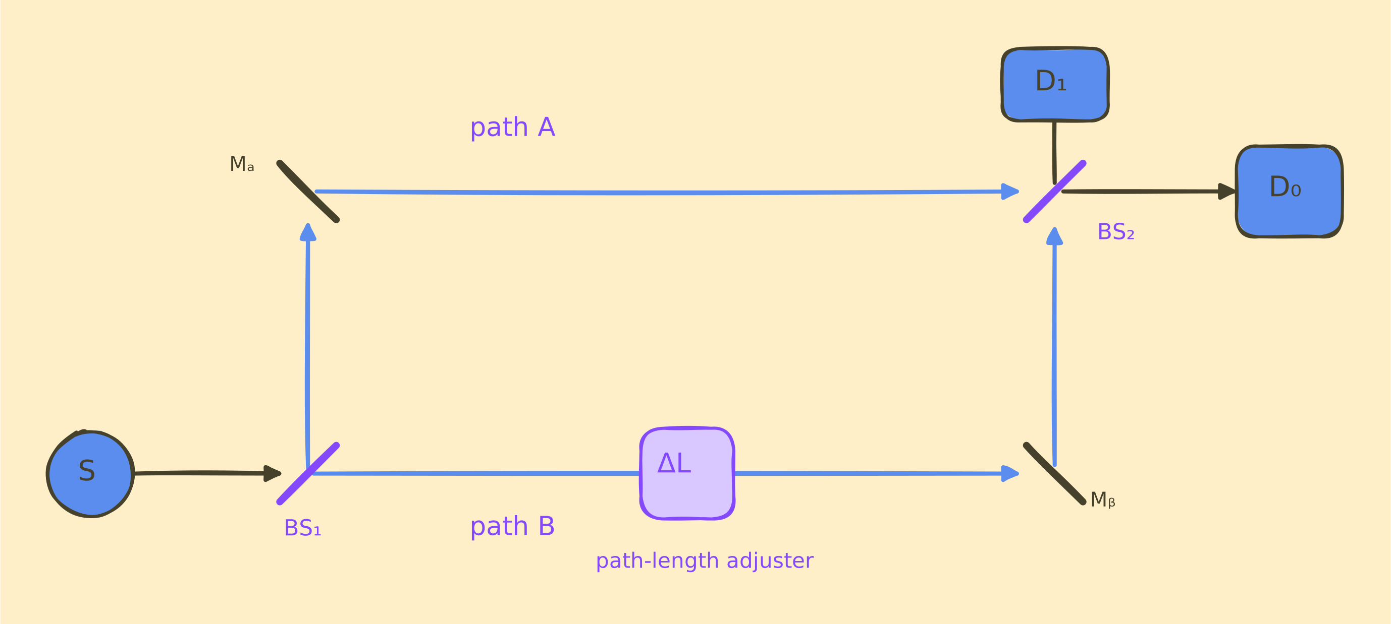
Our question is:
Given what happens along each path, what fraction of the particles will arrive at each detector?
The adjustable rectangle in path \(B\) does not move either mirror. It represents a phase-shifting element designed to leave the outgoing beam on the same geometric route. For light, a transparent material makes propagation through a segment behave as though the path were longer: a segment of geometric length \(\ell\) and refractive index \(n\) contributes the effective optical length \(n\ell\). Changing the material or the thickness traversed changes that effective length without redirecting the beam away from \(M_B\).
Let the effective path lengths be \(L_A\) and \(L_B\). First make them equal, so the apparatus can be adjusted until every particle is detected at \(D_0\). Then use the element to change the effective length of path \(B\) while leaving its geometric route and path \(A\) fixed. The independently controlled effective path-length difference is
\[\Delta L=L_B-L_A.\]For each chosen \(\Delta L\), send many particles through the apparatus. The detection frequency at a detector means the number of clicks there divided by the total number of particles sent. These measured frequencies estimate the detection probabilities. As \(\Delta L\) is varied, they change continuously and eventually repeat:
| Additional effective length in path \(B\) | Detection probabilities |
|---|---|
| \(\Delta L=0\) | \(P(D_0)=1,\quad P(D_1)=0\) |
| \(\Delta L=\lambda/4\) | \(P(D_0)=P(D_1)=1/2\) |
| \(\Delta L=\lambda/2\) | \(P(D_0)=0,\quad P(D_1)=1\) |
| \(\Delta L=\lambda\) | \(P(D_0)=1,\quad P(D_1)=0\) |
Individual particles produce individual detector clicks. The repeating pattern appears only after many trials.
The symbol \(\lambda\) denotes the smallest positive change in \(\Delta L\) after which the detector statistics repeat. There is no recursive definition: the experimenter sets and measures \(\Delta L\), then uses the resulting detector frequencies to measure \(\lambda\) once. After that calibration, the measured \(\lambda\) predicts the probabilities for new choices of \(\Delta L\).
Let \(\theta_A\) and \(\theta_B\) denote the phases accumulated along the two paths. Only their difference affects the detector probabilities. Because path \(A\) remains fixed while the adjuster changes path \(B\), define
\[\theta :=\theta_{\mathrm{relative}} :=\theta_B-\theta_A =\frac{2\pi\Delta L}{\lambda}.\]Throughout the rest of this post, \(\theta\) always means this relative phase. At this stage it means “position within the repeating interference pattern.”
More generally, changes in travel time or potential along a path can move the same interference pattern. Two successive changes shift the pattern by the sum of their individual amounts, so their phase changes add:
\[\theta_{\mathrm{combined}}=\theta_1+\theta_2.\]This is why phase is said to accumulate along a path: consecutive portions of the journey contribute consecutive shifts within the observed cycle.
If both paths are changed by the same amount, \(\theta_A\) and \(\theta_B\) increase equally, so their difference \(\theta\) and the detector statistics do not change.
Operationally, phase belongs to a path’s contribution to the later interference. Its meaning is revealed only when that contribution is compared with another path.
We compare four apparatus configurations:
\[\begin{aligned} C_0&:=\text{both paths enter the second beam splitter},\\ C_A&:=\text{only path }A\text{ enters the second beam splitter},\\ C_B&:=\text{only path }B\text{ enters the second beam splitter},\\ C_p&:=\text{the paths are detected before the second beam splitter}. \end{aligned}\]Let \(C\) denote the chosen configuration:
\[C\in\mathcal C, \qquad \mathcal C:=\{C_0,C_A,C_B,C_p\}.\]In configuration \(C_p\), let the recorded path be the random variable
\[X\in\Omega, \qquad \Omega:=\{A,B\}.\]The first beam splitter is balanced, so the measured path frequencies are
\[P(X=A\mid C=C_p,\theta) =P(X=B\mid C=C_p,\theta) =\frac12.\]The separate-input configurations calibrate the second beam splitter:
\[\begin{aligned} P(D_0\mid C=C_A,\theta) &=P(D_1\mid C=C_A,\theta)=\frac12,\\ P(D_0\mid C=C_B,\theta) &=P(D_1\mid C=C_B,\theta)=\frac12. \end{aligned}\]2. Why are these probabilities not enough?
Suppose that, in configuration \(C_0\), every trial possesses one exclusive path value \(X\in\Omega\) and the single-path calibrations can be transferred unchanged into that configuration. The assumptions are
\[\begin{aligned} P(X=A\mid C=C_0,\theta) &=P(X=A\mid C=C_p,\theta)=\frac12,\\ P(X=B\mid C=C_0,\theta) &=P(X=B\mid C=C_p,\theta)=\frac12,\\ P(D_0\mid X=A,C=C_0,\theta) &=P(D_0\mid C=C_A,\theta)=\frac12,\\ P(D_0\mid X=B,C=C_0,\theta) &=P(D_0\mid C=C_B,\theta)=\frac12. \end{aligned}\]Because \(X=A\) and \(X=B\) are mutually exclusive and exhaustive within this proposed model, the law of total probability gives
\[\begin{aligned} P(D_0\mid C=C_0,\theta) &=\sum_{x\in\Omega} P(D_0\mid X=x,C=C_0,\theta)P(X=x\mid C=C_0,\theta)\\ &=\frac12\cdot\frac12+\frac12\cdot\frac12\\ &=\frac12. \end{aligned}\]But the measured probability in the same configuration varies with \(\theta\):
\[P(D_0\mid C=C_0,\theta) =\cos^2\left(\frac\theta2\right).\]For example,
\[P(D_0\mid C=C_0,\theta=\pi)=0\ne\frac12.\]The conjunction of the transfer assumptions has failed: probabilities measured after changing the apparatus to \(C_A\), \(C_B\), or \(C_p\) cannot be inserted as though they were conditional probabilities inside \(C_0\).
3. Can one state and recombination rule predict \(C_p\) and \(C_0\)?
The subscript in \(F_0\) refers to detector \(D_0\).
We want a \(\theta\)-dependent path state \(s_\theta:\Omega\to\mathbb R\) and a fixed detector rule \(F_0:\mathbb R^2\to\mathbb R_{\ge0}\) satisfying
\[P(D_0\mid C=C_0,\theta) =F_0\!\left(s_\theta(A),s_\theta(B)\right) =\cos^2\left(\frac\theta2\right).\]In this notation, the rejected classical model used
\[\begin{aligned} s_\theta^{\mathrm{cl}}(A) &:=P(X=A\mid C=C_p,\theta),\\ s_\theta^{\mathrm{cl}}(B) &:=P(X=B\mid C=C_p,\theta),\\ F_0^{\mathrm{cl}}(u,v) &:=P(D_0\mid C=C_A,\theta)u\\ &\quad+P(D_0\mid C=C_B,\theta)v. \end{aligned}\]First test real path values and a squared-linear rule, so that the two terms can cancel while the result remains nonnegative:
\[\begin{aligned} s_\theta(x) &\in \left\{ -\sqrt{P(X=x\mid C=C_p,\theta)}, +\sqrt{P(X=x\mid C=C_p,\theta)} \right\},\\ &=\left\{-\frac1{\sqrt2},+\frac1{\sqrt2}\right\}, \qquad x\in\Omega,\\ F_0(u,v) &:=\left( \sqrt{P(D_0\mid C=C_A,\theta)}\,u +\sqrt{P(D_0\mid C=C_B,\theta)}\,v \right)^2. \end{aligned}\]The state \(s_\theta\) above is inferred from the path frequencies measured in \(C_p\). Independently, the configurations \(C_A\) and \(C_B\) calibrate how \(F_0\) responds when only one path enters the second beam splitter. If \(X\) is extended here to label that input path, then passing \((1,0)\) means setting
\[P(X=A\mid C=C_A,\theta)=1, \qquad P(X=B\mid C=C_A,\theta)=0,\]while passing \((0,1)\) means setting
\[P(X=A\mid C=C_B,\theta)=0, \qquad P(X=B\mid C=C_B,\theta)=1.\]These are single-path calibration inputs, not possible values of the two-path state \(s_\theta\). They determine the rule \(F_0\) independently:
\[\begin{aligned} F_0(1,0) &=P(D_0\mid C=C_A,\theta)=\frac12,\\ F_0(0,1) &=P(D_0\mid C=C_B,\theta)=\frac12. \end{aligned}\]The calibrated rule is then applied to the \(C_p\)-derived input \(\bigl(s_\theta(A),s_\theta(B)\bigr)\) to predict \(C_0\).
Expanding the definition of \(F_0\) gives
\[\begin{aligned} F_0\!\left(s_\theta(A),s_\theta(B)\right) &=P(D_0\mid C=C_A,\theta)s_\theta(A)^2\\ &\quad+P(D_0\mid C=C_B,\theta)s_\theta(B)^2\\ &\quad+2\sqrt{ P(D_0\mid C=C_A,\theta) P(D_0\mid C=C_B,\theta) }\,s_\theta(A)s_\theta(B)\\ &=\frac12+s_\theta(A)s_\theta(B). \end{aligned}\]Because \(s_\theta(A),s_\theta(B)\in\{-1/\sqrt2,+1/\sqrt2\}\),
\[s_\theta(A)s_\theta(B) \in\left\{-\frac12,+\frac12\right\}, \qquad F_0\!\left(s_\theta(A),s_\theta(B)\right)\in\{0,1\}.\]But
\[P(D_0\mid C=C_0,\theta=\pi/2)=\frac12 \notin\{0,1\},\]so no such real-valued family \(s_\theta\) and fixed rule \(F_0\) can satisfy both requirements.
The missing information is a continuously variable relation between the two path contributions. Replace the real-valued path state \(s_\theta\) by
\[\boldsymbol\psi_\theta:\Omega\longrightarrow\mathbb R^2.\]Choose path \(A\) as the phase reference, so \(\theta_A=0\) and \(\theta_B=\theta\). Define \(\boldsymbol\psi_\theta\) by
\[\begin{aligned} \boldsymbol\psi_\theta(A) &:=\sqrt{P(X=A\mid C=C_p,\theta)} \begin{pmatrix} 1\\ 0 \end{pmatrix},\\ \boldsymbol\psi_\theta(B) &:=\sqrt{P(X=B\mid C=C_p,\theta)} \begin{pmatrix} \cos\theta\\ \sin\theta \end{pmatrix}, \end{aligned}\]Their squared lengths reproduce the path probabilities:
\[\begin{aligned} \lVert\boldsymbol\psi_\theta(A)\rVert^2 &=P(X=A\mid C=C_p,\theta)=\frac12,\\ \lVert\boldsymbol\psi_\theta(B)\rVert^2 &=P(X=B\mid C=C_p,\theta)=\frac12. \end{aligned}\]Their angle retains the additional quantity measured by the interference experiment:
\[\frac{ \boldsymbol\psi_\theta(A)\cdot \boldsymbol\psi_\theta(B)} {\lVert\boldsymbol\psi_\theta(A)\rVert \lVert\boldsymbol\psi_\theta(B)\rVert} =\cos\theta.\]Correspondingly, replace \(F_0:\mathbb R^2\to\mathbb R_{\ge0}\) by
\[\mathcal F_0:\mathbb R^2\times\mathbb R^2 \longrightarrow\mathbb R_{\ge0},\]where
\[\mathcal F_0(\boldsymbol u,\boldsymbol v) :=\left\lVert \sqrt{P(D_0\mid C=C_A,\theta)}\,\boldsymbol u +\sqrt{P(D_0\mid C=C_B,\theta)}\,\boldsymbol v \right\rVert^2.\]The two calibration probabilities are \(1/2\) for every \(\theta\), so this is one fixed function. Applied to the new path state,
\[\begin{aligned} \mathcal F_0\!\left( \boldsymbol\psi_\theta(A), \boldsymbol\psi_\theta(B) \right) &=\frac12\left\lVert \boldsymbol\psi_\theta(A)+ \boldsymbol\psi_\theta(B) \right\rVert^2\\ &=\frac12(1+\cos\theta)\\ &=P(D_0\mid C=C_0,\theta). \end{aligned}\]This already answers the original question about \(D_0\). The state \(\boldsymbol\psi_\theta\) retains the path probabilities and relative phase; the rule \(\mathcal F_0\) uses that state to produce \(P(D_0\mid C=C_0,\theta)\). Nothing else is required if \(D_0\) is the only output we want to predict.
This motivates the definition:
A path amplitude is a two-dimensional real vector whose squared length gives the probability of that path in configuration \(C_p\) and whose direction retains the phase needed to predict later interference.
3.1. How does a basis describe the path state?
The successful path states form
\[(\mathbb R^2)^\Omega :=\{\boldsymbol\psi\mid\boldsymbol\psi:\Omega\to\mathbb R^2\}.\]With pointwise vector addition and scalar multiplication, \((\mathbb R^2)^\Omega\) is the path-state space. Its elements are complete path states; a basis is only a particular set of elements used to expand them.
Because \(\Omega=\{A,B\}\), the coordinate map
\[\begin{aligned} \operatorname{coord}_{(A,B)} &:(\mathbb R^2)^\Omega\longrightarrow\mathbb R^4,\\ \operatorname{coord}_{(A,B)}(\boldsymbol\psi) &:= \begin{pmatrix} \boldsymbol\psi(A)\\ \boldsymbol\psi(B) \end{pmatrix} \end{aligned}\]is a linear isomorphism:
\[(\mathbb R^2)^\Omega \cong \mathbb R^4.\]Thus a path state may be represented as a block vector with two \(\mathbb R^2\) entries. For example,
\[\operatorname{coord}_{(A,B)}(\boldsymbol\psi_\theta) = \begin{pmatrix} \sqrt{P(X=A\mid C=C_p,\theta)} \begin{pmatrix}1\\0\end{pmatrix}\\[6pt] \sqrt{P(X=B\mid C=C_p,\theta)} \begin{pmatrix}\cos\theta\\\sin\theta\end{pmatrix} \end{pmatrix} \in\mathbb R^4.\]For each \(X\in\Omega\), define the scalar-valued path selector
\[\begin{aligned} e_X&:\Omega\longrightarrow\mathbb R,\\ e_X(Y)&:= \begin{cases} 1,&Y=X,\\ 0,&Y\ne X, \end{cases} \qquad Y\in\Omega. \end{aligned}\]Thus \(e_A\) selects path \(A\) and \(e_B\) selects path \(B\). Define the standard basis vectors of each path’s amplitude plane by
\[\boldsymbol r_1,\boldsymbol r_2\in\mathbb R^2, \qquad \boldsymbol r_1:= \begin{pmatrix}1\\0\end{pmatrix}, \qquad \boldsymbol r_2:= \begin{pmatrix}0\\1\end{pmatrix}.\]Their combination is the function
\[\begin{aligned} e_X\otimes\boldsymbol u&:\Omega\longrightarrow\mathbb R^2,\\ (e_X\otimes\boldsymbol u)(Y) &:=e_X(Y)\boldsymbol u, \end{aligned} \qquad X,Y\in\Omega, \quad \boldsymbol u\in\mathbb R^2.\]Therefore, by the probability rule for amplitudes,
\[\left\{ e_A\otimes\boldsymbol r_1, e_A\otimes\boldsymbol r_2, e_B\otimes\boldsymbol r_1, e_B\otimes\boldsymbol r_2 \right\}\]is a basis of \((\mathbb R^2)^\Omega\). The previously defined state has the explicit expansion
\[\begin{aligned} \boldsymbol\psi_\theta &=e_A\otimes\boldsymbol\psi_\theta(A) +e_B\otimes\boldsymbol\psi_\theta(B)\\ &=\sqrt{P(X=A\mid C=C_p,\theta)} \left(e_A\otimes\boldsymbol r_1\right)\\ &\quad+0\left(e_A\otimes\boldsymbol r_2\right)\\ &\quad+\sqrt{P(X=B\mid C=C_p,\theta)}\cos\theta \left(e_B\otimes\boldsymbol r_1\right)\\ &\quad+\sqrt{P(X=B\mid C=C_p,\theta)}\sin\theta \left(e_B\otimes\boldsymbol r_2\right). \end{aligned}\]More generally, for \(\boldsymbol u,\boldsymbol v\in\mathbb R^2\),
\[\boldsymbol\psi =e_A\otimes\boldsymbol u+e_B\otimes\boldsymbol v \quad\Longrightarrow\quad \boldsymbol\psi(A)=\boldsymbol u, \quad \boldsymbol\psi(B)=\boldsymbol v.\]Thus the earlier detector rule becomes
\[\begin{aligned} \mathcal F_0(\boldsymbol u,\boldsymbol v) &=\left\lVert \sqrt{P(D_0\mid C=C_A,\theta)}\,\boldsymbol u +\sqrt{P(D_0\mid C=C_B,\theta)}\,\boldsymbol v \right\rVert^2. \end{aligned}\]In \(C_A\) only the path-\(A\) component is present; in \(C_B\) only the path-\(B\) component is present. Use the concrete unit amplitude
\[\boldsymbol r_1= \begin{pmatrix}1\\0\end{pmatrix}, \qquad \lVert\boldsymbol r_1\rVert^2=1.\]Then
\[\begin{aligned} \mathcal F_0(\boldsymbol r_1,\boldsymbol 0) &=P(D_0\mid C=C_A,\theta)\lVert\boldsymbol r_1\rVert^2\\ &=P(D_0\mid C=C_A,\theta),\\ \mathcal F_0(\boldsymbol 0,\boldsymbol r_1) &=P(D_0\mid C=C_B,\theta)\lVert\boldsymbol r_1\rVert^2\\ &=P(D_0\mid C=C_B,\theta), \end{aligned}\]The definition of \(\mathcal F_0\) already assumes that a common rotation of the amplitude plane changes no probability. For every \(R\in\mathbb R^{2\times2}\) satisfying \(R^{\mathsf T}R=I\) and \(\det R=1\),
\[\mathcal F_0(R\boldsymbol u,R\boldsymbol v) =\mathcal F_0(\boldsymbol u,\boldsymbol v).\]Therefore every unit direction gives the same single-path result. In particular, because \(\lVert\boldsymbol r_2\rVert^2=1\),
\[\begin{aligned} \mathcal F_0(\boldsymbol r_2,\boldsymbol 0) &=P(D_0\mid C=C_A,\theta),\\ \mathcal F_0(\boldsymbol 0,\boldsymbol r_2) &=P(D_0\mid C=C_B,\theta). \end{aligned}\]Thus testing \(\boldsymbol r_2\) would add no information. Without this rotational-symmetry assumption, the two basis directions and their linear combinations would have to be calibrated separately.
The first line evaluates \(\mathcal F_0\) on the ordered path-amplitude pair \((\boldsymbol r_1,\boldsymbol 0)\) used in \(C_A\); the second uses \((\boldsymbol 0,\boldsymbol r_1)\) in \(C_B\). Applying the inverse coordinate map defines the corresponding calibration path states \(\boldsymbol\psi_{C_A}\) and \(\boldsymbol\psi_{C_B}\):
\[\begin{aligned} \boldsymbol\psi_{C_A} &:= \operatorname{coord}_{(A,B)}^{-1} \begin{pmatrix} \boldsymbol r_1\\ \boldsymbol 0 \end{pmatrix} &=e_A\otimes\boldsymbol r_1,\\[6pt] \boldsymbol\psi_{C_B} &:= \operatorname{coord}_{(A,B)}^{-1} \begin{pmatrix} \boldsymbol 0\\ \boldsymbol r_1 \end{pmatrix} &=e_B\otimes\boldsymbol r_1. \end{aligned}\]Their squared component lengths express the single-path inputs:
\[\begin{aligned} P(X=A\mid C=C_A,\theta) &=\lVert\boldsymbol\psi_{C_A}(A)\rVert^2=1, &\qquad P(X=B\mid C=C_A,\theta) &=\lVert\boldsymbol\psi_{C_A}(B)\rVert^2=0,\\ P(X=A\mid C=C_B,\theta) &=\lVert\boldsymbol\psi_{C_B}(A)\rVert^2=0, & P(X=B\mid C=C_B,\theta) &=\lVert\boldsymbol\psi_{C_B}(B)\rVert^2=1. \end{aligned}\]These calibration states are distinct from the two-path state \(\boldsymbol\psi_\theta\), whose component lengths come from \(C_p\) and which is used to predict the detector probabilities in \(C_0\).
3.2. Can one rule predict both detector outputs?
The apparatus also contains \(D_1\). The rule \(\mathcal F_0\) returns only the probability at \(D_0\) and discards the resulting output amplitude. We could define a separate rule for \(D_1\), but then the two rules would not express that both outputs come from the same second beam splitter.
We therefore generalize \(\mathcal F_0\) to one map that returns an amplitude for every detector. Squared lengths of those amplitudes will give both detector probabilities, and the output amplitudes remain available if another component is placed after the beam splitter.
Define the detector-label set
\[\Delta:=\{D_0,D_1\}.\]In \(C_A\), only the amplitude from path \(A\) enters the second beam splitter. In \(C_B\), only the amplitude from path \(B\) enters it. We now want those two measurements to predict what happens in \(C_0\), where both amplitudes enter together. To combine the two single-path responses, assume that the beam splitter acts linearly.
Therefore define the beam-splitter map and its output by
\[\begin{aligned} (\mathbb R^2)^\Delta &:=\{\boldsymbol v:\Delta\to\mathbb R^2\},\\ M_{\mathrm{BS}}&:(\mathbb R^2)^\Omega\to(\mathbb R^2)^\Delta,\\ \boldsymbol\phi_\theta&:=M_{\mathrm{BS}}\boldsymbol\psi_\theta, \end{aligned}\]Define the detector-coordinate map
\[\begin{aligned} \operatorname{coord}_{(D_0,D_1)} &:(\mathbb R^2)^\Delta\longrightarrow\mathbb R^4,\\ \operatorname{coord}_{(D_0,D_1)}(\boldsymbol\phi) &:= \begin{pmatrix} \boldsymbol\phi(D_0)\\ \boldsymbol\phi(D_1) \end{pmatrix}. \end{aligned}\]For each detector label \(D\in\Delta\) and path label \(X\in\Omega\), let \((M_{\mathrm{BS}})_{D,X}\) denote the coefficient mapping the amplitude from path \(X\) to detector \(D\).
The same two normalized inputs now calibrate the response at both detectors. In detector coordinates,
\[\begin{aligned} \operatorname{coord}_{(D_0,D_1)} \!\left(M_{\mathrm{BS}}(e_A\otimes\boldsymbol r_1)\right) &= \begin{pmatrix} (M_{\mathrm{BS}})_{D_0,A}\boldsymbol r_1\\ (M_{\mathrm{BS}})_{D_1,A}\boldsymbol r_1 \end{pmatrix},\\[8pt] \operatorname{coord}_{(D_0,D_1)} \!\left(M_{\mathrm{BS}}(e_B\otimes\boldsymbol r_1)\right) &= \begin{pmatrix} (M_{\mathrm{BS}})_{D_0,B}\boldsymbol r_1\\ (M_{\mathrm{BS}})_{D_1,B}\boldsymbol r_1 \end{pmatrix}. \end{aligned}\]For every \((D,X)\in\Delta\times\Omega\),
\[\begin{aligned} \left\lVert (M_{\mathrm{BS}})_{D,X}\boldsymbol r_1 \right\rVert^2 &=\lvert(M_{\mathrm{BS}})_{D,X}\rvert^2 \lVert\boldsymbol r_1\rVert^2\\ &=\lvert(M_{\mathrm{BS}})_{D,X}\rvert^2. \end{aligned}\]Therefore
\[\begin{aligned} P(D_0\mid C=C_A,\theta) &=\left\lVert(M_{\mathrm{BS}})_{D_0,A}\boldsymbol r_1\right\rVert^2\\ &=\lvert(M_{\mathrm{BS}})_{D_0,A}\rvert^2=\frac12,\\ P(D_1\mid C=C_A,\theta) &=\left\lVert(M_{\mathrm{BS}})_{D_1,A}\boldsymbol r_1\right\rVert^2\\ &=\lvert(M_{\mathrm{BS}})_{D_1,A}\rvert^2=\frac12,\\ P(D_0\mid C=C_B,\theta) &=\left\lVert(M_{\mathrm{BS}})_{D_0,B}\boldsymbol r_1\right\rVert^2\\ &=\lvert(M_{\mathrm{BS}})_{D_0,B}\rvert^2=\frac12,\\ P(D_1\mid C=C_B,\theta) &=\left\lVert(M_{\mathrm{BS}})_{D_1,B}\boldsymbol r_1\right\rVert^2\\ &=\lvert(M_{\mathrm{BS}})_{D_1,B}\rvert^2=\frac12. \end{aligned}\]For each detector output, choose the axes of its amplitude plane so that the coefficient from input \(A\) is positive. At \(\theta=0\),
\[\boldsymbol\psi_0(A) =\boldsymbol\psi_0(B) =\frac{\boldsymbol r_1}{\sqrt2}.\]Therefore linearity gives, for each \(D\in\Delta\),
\[\boldsymbol\phi_0(D) =\frac{ (M_{\mathrm{BS}})_{D,A}+(M_{\mathrm{BS}})_{D,B} }{\sqrt2}\,\boldsymbol r_1.\]The experiment gives
\[P(D_0\mid C=C_0,\theta=0)=1, \qquad P(D_1\mid C=C_0,\theta=0)=0.\]By the probability rule for amplitudes,
\[\begin{aligned} 1 &=\lVert\boldsymbol\phi_0(D_0)\rVert^2 =\frac12\left| (M_{\mathrm{BS}})_{D_0,A}+(M_{\mathrm{BS}})_{D_0,B} \right|^2,\\ 0 &=\lVert\boldsymbol\phi_0(D_1)\rVert^2 =\frac12\left| (M_{\mathrm{BS}})_{D_1,A}+(M_{\mathrm{BS}})_{D_1,B} \right|^2. \end{aligned}\]Every coefficient has magnitude \(1/\sqrt2\). The first equality therefore requires the two coefficients at \(D_0\) to have the same sign; the second requires those at \(D_1\) to have opposite signs. Hence
\[(M_{\mathrm{BS}})_{D_0,A}=(M_{\mathrm{BS}})_{D_1,A}=\frac1{\sqrt2}, \qquad (M_{\mathrm{BS}})_{D_0,B}=(M_{\mathrm{BS}})_{D_0,A}, \qquad (M_{\mathrm{BS}})_{D_1,B}=-(M_{\mathrm{BS}})_{D_1,A}.\]Therefore
\[M_{\mathrm{BS}} =\frac1{\sqrt2} \begin{pmatrix} 1&1\\ 1&-1 \end{pmatrix}.\]This matrix was not chosen independently of the experiment: the single-input calibrations fixed the magnitudes \(1/\sqrt2\), and the constructive and destructive outputs at \(\theta=0\) fixed the relative signs.
Applying \(M_{\mathrm{BS}}\) gives
\[\begin{aligned} \boldsymbol\phi_\theta(D_0) &=\frac{ \boldsymbol\psi_\theta(A)+ \boldsymbol\psi_\theta(B)} {\sqrt2},\\ \boldsymbol\phi_\theta(D_1) &=\frac{ \boldsymbol\psi_\theta(A)- \boldsymbol\psi_\theta(B)} {\sqrt2}. \end{aligned}\]For \(D_0\), the new map reproduces the earlier rule exactly:
\[\mathcal F_0\!\left( \boldsymbol\psi_\theta(A), \boldsymbol\psi_\theta(B) \right) =\lVert\boldsymbol\phi_\theta(D_0)\rVert^2.\]The detector probabilities are the squared lengths of these output amplitudes:
\[\begin{aligned} P(D_0\mid C=C_0,\theta) &=\lVert\boldsymbol\phi_\theta(D_0)\rVert^2 =\frac12(1+\cos\theta) =\cos^2\left(\frac\theta2\right),\\ P(D_1\mid C=C_0,\theta) &=\lVert\boldsymbol\phi_\theta(D_1)\rVert^2 =\frac12(1-\cos\theta) =\sin^2\left(\frac\theta2\right). \end{aligned}\]Thus the same state predicts both the path probabilities and the interference probabilities. The state alone does not specify a probability until the experimental configuration specifies which output amplitudes are to be calculated.
4. Why use complex numbers?
The real two-dimensional amplitudes already reproduce the experiment. Complex numbers give the same vector addition, length, and rotation with less notation.
Identify
\[\begin{pmatrix} x\\ y \end{pmatrix} \longleftrightarrow x+iy.\]Then
\[\begin{aligned} \boldsymbol\psi_\theta(A) &\longleftrightarrow \psi_\theta(A) =\sqrt{P(X=A\mid C=C_p,\theta)},\\ \boldsymbol\psi_\theta(B) &\longleftrightarrow \psi_\theta(B) =\sqrt{P(X=B\mid C=C_p,\theta)}\,e^{i\theta}. \end{aligned}\]The path state is the function
\[\psi_\theta:\Omega\to\mathbb C\]or equivalently the vector
\[\psi_\theta = \begin{pmatrix} \sqrt{P(X=A\mid C=C_p,\theta)}\\ \sqrt{P(X=B\mid C=C_p,\theta)}\,e^{i\theta} \end{pmatrix}.\]The vector space of two-path states is
\[\mathcal H :=\mathbb C^\Omega =\{\psi:\Omega\to\mathbb C\}.\]The beam-splitter map has the same matrix in complex notation:
\[M_{\mathrm{BS}} =\frac1{\sqrt2} \begin{pmatrix} 1&1\\ 1&-1 \end{pmatrix},\]so
\[M_{\mathrm{BS}}\psi_\theta =\frac12 \begin{pmatrix} 1+e^{i\theta}\\ 1-e^{i\theta} \end{pmatrix}.\]The detector probabilities are
\[\begin{aligned} P(D_0\mid C=C_0,\theta) &=\lvert(M_{\mathrm{BS}}\psi_\theta)(D_0)\rvert^2,\\ P(D_1\mid C=C_0,\theta) &=\lvert(M_{\mathrm{BS}}\psi_\theta)(D_1)\rvert^2. \end{aligned}\]5. Where does the group structure enter?
If the adjuster adds a further relative phase \(\delta\), it changes the state by
\[\Phi_\delta: \begin{pmatrix} \psi(A)\\ \psi(B) \end{pmatrix} \longmapsto \begin{pmatrix} \psi(A)\\ e^{i\delta}\psi(B) \end{pmatrix}.\]Successive adjustments satisfy
\[\Phi_{\delta_2}\circ\Phi_{\delta_1} =\Phi_{\delta_1+\delta_2}, \qquad \Phi_0=\operatorname{id}.\]The unit complex numbers form the group
\[U(1) =\{e^{i\delta}:\delta\in\mathbb R\} \cong SO(2).\]In the equivalent real description, the rotation generator is
\[J= \begin{pmatrix} 0&-1\\ 1&0 \end{pmatrix}, \qquad J^2=-I,\]and
\[R(\delta)=e^{\delta J}.\]Under the identification with complex numbers, multiplication by \(J\) becomes multiplication by \(i\). The imaginary unit is therefore the concise representation of the real rotation structure required to retain continuously varying phase.
Multiplying the entire state by the same phase does not affect any probability:
\[\lvert(M_{\mathrm{BS}}(e^{i\chi}\psi))(D_j)\rvert^2 =\lvert e^{i\chi}(M_{\mathrm{BS}}\psi)(D_j)\rvert^2 =\lvert(M_{\mathrm{BS}}\psi)(D_j)\rvert^2.\]Here \(j\in\{0,1\}\). The angle \(\chi\) is called a global phase; only relative phases affect the detector statistics.
The construction above derives a state that predicts both path and detector measurements and a beam-splitter map calibrated from the experiment. The next question—how such a state changes with time—is developed in From Quantum State to the Schrödinger Equation.