
From Free Fall to Curved Spacetime
Physics ·From Light Signals to Spacetime constructed the rule relating observations made by inertial laboratories. We now begin with a laboratory near Earth and ask:
Can one rule predict how freely released objects move, how clocks at different heights compare, and how light travels?
We will first solve the falling-object problem without geometry or gravitational mass. We will then ask whether the measurements admit one gravitational rule that works for different test objects, and introduce curved spacetime only when a single observational model must describe falling objects, clocks, and light.
1. What does a released object do near Earth?
Choose a vertical position coordinate \(z\) that increases upward. Release a small object in an evacuated chamber and record its position with the chamber’s clocks. Over a sufficiently small height and time, the observations are described by
\[z(t)=z_0+u_0t-\frac12gt^2,\]where \(z_0\) is its position at \(t=0\), \(u_0\) is its initial upward velocity, and \(g\) is a measured positive constant. Differentiating twice gives
\[\frac{d^2z}{dt^2}=-g.\]This rule already predicts the position of that object. If it is released from rest at height \(h\) above the floor, then \(z_0=h\) and \(u_0=0\). It reaches the floor when
\[0=h-\frac12gt_{\mathrm{fall}}^2,\]so
\[t_{\mathrm{fall}}=\sqrt{\frac{2h}{g}}.\]Now repeat the evacuated-chamber experiment with objects made from different materials. Give them the same initial position and velocity:
| Released object | Measured vertical acceleration |
|---|---|
| Aluminum sphere | \(-g\) |
| Glass sphere | \(-g\) |
| Dense metal sphere | \(-g\) |
Within experimental precision, the same value of \(g\) describes every tested object. Objects released with the same initial conditions therefore follow the same trajectory, regardless of their material or mass. This conclusion applies to sufficiently small test objects whose own influence on Earth can be neglected.
The original drop problem is solved for every such object. We did not need either inertial mass or gravitational mass. Now ask for a different prediction:
How strong must a spring or floor be to support different objects at different locations?
2. How strong must the support be?
The earlier mechanics construction defined relative inertial mass by comparing the accelerations of two objects under the same controlled interaction:
\[\frac{m_{\mathrm{i},A}}{m_{\mathrm{i},B}} :=\frac{a_B}{a_A}.\]The subscript \(\mathrm{i}\) labels the inertial mass already calibrated in that separate experiment. Once those masses were calibrated, the same construction defined force by
\[F:=m_{\mathrm{i}}a.\]Suppose those experiments assign object \(A\) an inertial mass of \(1\ \mathrm{kg}\) and object \(B\) an inertial mass of \(2\ \mathrm{kg}\).
Now construct the support experiment. Fix one end of a calibrated spring to the ceiling and attach a test object \(X\) to its lower end. Wait until the object is at rest. Let \(x_X\) be the spring’s downward extension from its natural length.
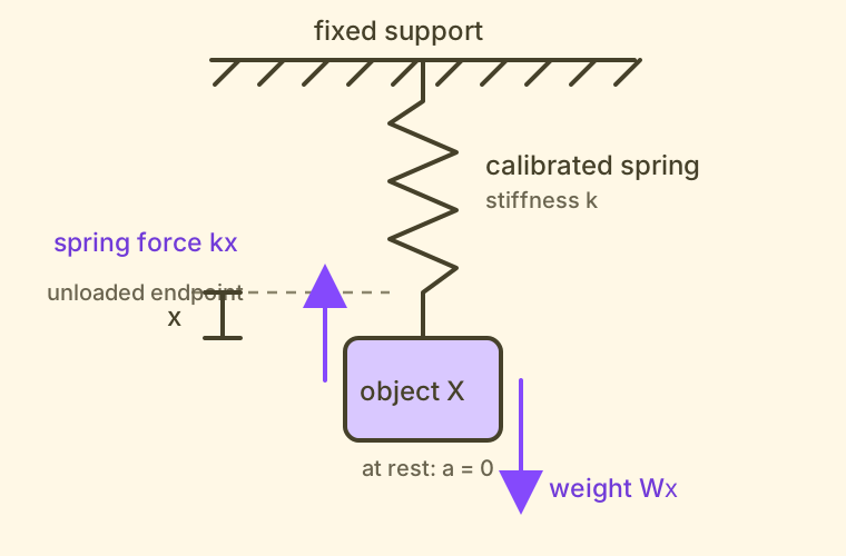
The drop rule tells us how \(X\) moves after release, but it does not predict the extension \(x_X\) while the spring holds it. Suppose the spring’s calibrated stiffness is \(k=100\ \mathrm{N/m}\). It pulls upward with magnitude \(kx_X\). Because the supported object has zero acceleration, the total force on it is zero. The downward gravitational force must therefore have the same magnitude:
\[W_X:=kx_X.\]Here \(W_X\) is the object’s weight at that location. This is an operational measurement of gravitational force: the calibrated spring force balances it.
Now repeat the measurement at two locations, \(L_1\) and \(L_2\). The following values illustrate the observed pattern:
| Object | Inertial mass | \(x\) at \(L_1\) | Weight at \(L_1\) | \(x\) at \(L_2\) | Weight at \(L_2\) |
|---|---|---|---|---|---|
| \(A\) | \(1\ \mathrm{kg}\) | \(0.098\ \mathrm{m}\) | \(9.8\ \mathrm{N}\) | \(0.095\ \mathrm{m}\) | \(9.5\ \mathrm{N}\) |
| \(B\) | \(2\ \mathrm{kg}\) | \(0.196\ \mathrm{m}\) | \(19.6\ \mathrm{N}\) | \(0.190\ \mathrm{m}\) | \(19.0\ \mathrm{N}\) |
There is not one numerical gravitational force shared by both objects. At either location, object \(B\) has twice the weight of object \(A\). But the ratio belonging to the pair of objects is stable:
\[\frac{W_A(L_1)}{W_B(L_1)} =\frac{W_A(L_2)}{W_B(L_2)} =\frac12.\]Experiments with other calibrated springs check that this ratio does not depend on the supporting apparatus. Experiments at other locations check that it does not depend on the local gravitational environment. When those checks succeed, we can assign the stable factor to the objects. Define relative passive gravitational mass by
\[\frac{m_{\mathrm{g},A}}{m_{\mathrm{g},B}} :=\frac{W_A(L)}{W_B(L)}\]when both weights are measured at the same location \(L\). Choosing one reference object fixes the overall gravitational-mass unit. “Passive” means that this quantity describes how strongly the test object responds to an existing gravitational environment. It does not yet describe how strongly the object would produce gravity if used as a source.
Once the object factors have been calibrated, divide them out of the measured weights. At location \(L\), define
\[\gamma(L):=\frac{W_X(L)}{m_{\mathrm{g},X}}.\]The measured stability of the weight ratios makes \(\gamma(L)\) independent of which test object \(X\) is used. It describes the location and source, while \(m_{\mathrm{g},X}\) describes the test object. Every separate weight measurement is now summarized by one reusable rule:
\[W_X(L)=m_{\mathrm{g},X}\gamma(L).\]This factorization does predictive work. After measuring \(\gamma(L)\) with one reference object, we can predict the extension of a spring of stiffness \(k\) supporting any object whose passive gravitational mass is known:
\[x_X(L)=\frac{m_{\mathrm{g},X}\gamma(L)}{k}.\]A floor supporting the same object must provide the upward force \(m_{\mathrm{g},X}\gamma(L)\). Thus the construction answers the question that free-fall acceleration alone could not answer.
What happens when the support is removed?
Now release \(A\) and \(B\) in the evacuated chamber at \(L_1\). Their measured accelerations are
| Released object | Inertial mass | Passive gravitational mass | Measured vertical acceleration |
|---|---|---|---|
| \(A\) | \(1\ \mathrm{kg}\) | \(1\) gravitational-mass unit | \(-9.8\ \mathrm{m/s^2}\) |
| \(B\) | \(2\ \mathrm{kg}\) | \(2\) gravitational-mass units | \(-9.8\ \mathrm{m/s^2}\) |
Assume that removing the support does not change the gravitational interaction itself. With \(z\) increasing upward, the gravitational force is \(-W_X\). The inertial rule and the weight rule therefore give
\[m_{\mathrm{i},X}a_X =-W_X =-m_{\mathrm{g},X}\gamma,\]and hence
\[a_X=-\gamma\frac{m_{\mathrm{g},X}}{m_{\mathrm{i},X}}.\]The observed equality of the accelerations says that \(m_{\mathrm{g}}/m_{\mathrm{i}}\) has the same value for every tested object. This proportionality is an empirical result: inertial mass was calibrated from acceleration under controlled nongravitational interactions, while passive gravitational mass was calibrated from weight ratios.
Choose the gravitational-mass unit so that one reference object has the same numerical inertial and passive gravitational mass. The universal proportionality then gives
\[m_{\mathrm{g}}=m_{\mathrm{i}},\]and \(\gamma(L_1)=9.8\ \mathrm{m/s^2}=g\). The larger gravitational force on \(B\) does not give it a larger acceleration because its inertial mass is larger by the same factor. After establishing this result, either mass symbol alone is sufficient for calculations; keeping them separate allowed the equality to be discovered rather than assumed.
3. What does an accelerometer measure while falling?
The balance experiment used a supported spring to measure weight. Now place the same kind of spring and test mass inside a box. This physical box, together with its clocks, measuring instruments, and test objects, is what we mean by a laboratory. Mark the spring’s extension when the box rests on the ground. The support prevents the box from following the falling trajectory, while the test mass pulls on the spring.
Now release the entire box. During free fall, the test mass and the box acquire the same downward acceleration. The spring relaxes toward its unstretched reading.
An accelerometer is an instrument that uses such internal forces to report acceleration relative to free fall. We must now distinguish two meanings of acceleration:
-
Coordinate acceleration depends on the viewpoint. We may say “the ball accelerates downward” or “the floor accelerates upward.”
-
Proper acceleration is measured by an accelerometer and does not depend on coordinates.
“Proper” means that the reading is obtained locally by an instrument moving along the box’s own path; it does not require tracking the box against distant markers or clocks. A zero reading identifies free fall, while a nonzero reading measures how strongly the box is being pushed away from free fall. The reading alone cannot tell whether that push comes from a rocket floor or from the ground.
| Motion of the box | Accelerometer reading |
|---|---|
| Resting on the ground | Approximately \(g\) upward |
| Falling freely | Approximately \(0\) |
| Far from gravitating bodies with engines off | Approximately \(0\) |
| Rocket accelerating upward in empty space | Rocket acceleration \(a\) upward |
The falling box changes position rapidly, yet its accelerometer reads zero. The box on the ground has constant position, yet its accelerometer does not read zero. Proper acceleration is therefore not the second derivative of an arbitrary position coordinate.
Now compare the freely falling box near Earth with a box coasting far from gravitating bodies, with its engines off. Both accelerometers read zero. In either box, nearby released objects remain approximately at rest relative to the box. This correspondence motivates the equivalence principle:
In a sufficiently small freely falling laboratory, nongravitational experiments obey the same local rules as in an inertial laboratory without gravity.
Here the inertial laboratory is the real, non-accelerating box far from gravity—not a laboratory that is absolutely at rest. “Sufficiently small” matters because Earth’s gravitational acceleration changes with position and direction. A single falling laboratory can remove the common acceleration at one place, but it cannot remove differences across an arbitrarily large region.
4. Can an accelerating rocket reproduce the falling observations?
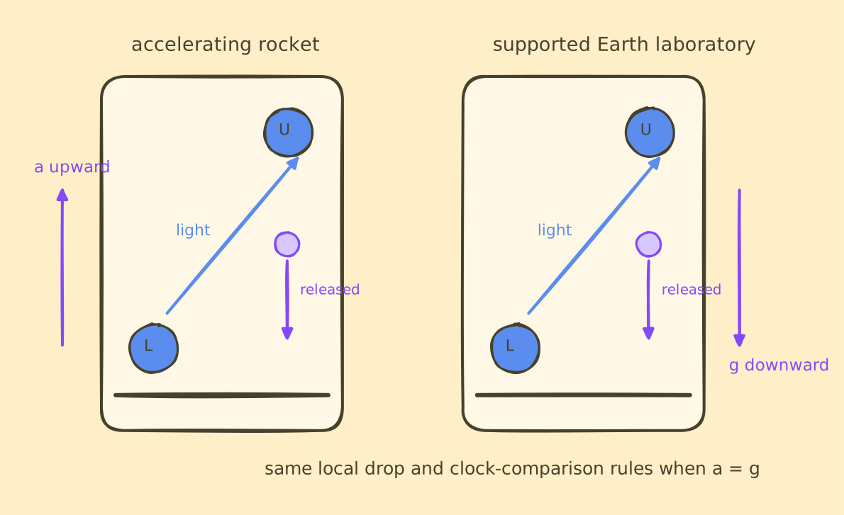
Consider a rocket far from gravitating bodies. Its engines make the floor accelerate upward with constant proper acceleration \(a\). Release a ball inside it. Immediately after release, the ball follows an inertial path while the floor accelerates toward it. Relative to rocket coordinates, the ball has the approximate update
\[\frac{d^2z}{dt^2}=-a.\]Set \(a=g\). Over a small enough region and duration, this is the same update measured for a released ball in the laboratory near Earth:
\[\frac{d^2z}{dt^2}=-g.\]In both laboratories, an accelerometer fixed to the floor reads upward acceleration \(g\). A released ball has zero proper acceleration, while the floor accelerates toward it, so the ball appears to fall. These local observations do not reveal whether the laboratory is supported near Earth or accelerating in empty space.
5. What does the rocket predict for clocks at different heights?
Place a light source at the rocket’s floor and a receiver a fixed proper distance \(h>0\) above it, measured by rulers at rest in the rocket. Let the source emit successive wave crests with frequency \(\nu_{\mathrm{lower}}\), meaning \(\nu_{\mathrm{lower}}\) crests per unit proper time of the lower clock. We want to predict how many crests arrive per unit proper time of the upper clock.
Whose coordinates describe the light and the rocket?
Choose an inertial frame in which the rocket is momentarily at rest when a crest leaves the floor. Let that emission occur at \(t=0\) and \(z=0\), with the receiver initially at \(z=h\). These coordinates belong to the inertial frame: after emission, the rocket accelerates through them. We do not keep changing frames to follow it.
Recall from the preceding post that light in vacuum travels at speed \(c\) in every inertial frame, independently of the source’s velocity. Therefore the upward crest follows
\[z_{\mathrm{light}}(t)=ct.\]The rocket’s acceleration changes the receiver’s trajectory. The arrival event is where that trajectory meets the light’s path.
How fast is the receiver moving when the light arrives?
We want the receiver’s upward speed \(\Delta v\) at reception, measured in the inertial frame where it started at rest. Its Taylor expansion about zero separation, \(h=0\), gives
\[\frac{\Delta v}{c} =\frac{ah}{c^2}+O\!\left(\frac{a^2h^2}{c^4}\right) =\epsilon+O(\epsilon^2),\]where \(\epsilon:=ah/c^2\). The omitted terms are small compared with the leading term when \(\epsilon\ll1\). Under this condition, we use \(\Delta v\approx ah/c\).
Why does a receding receiver count fewer crests?
First solve a separate special-relativistic problem. A source at rest in an inertial frame emits light upward at frequency \(\nu_0\). In one emission period \(1/\nu_0\), the preceding crest travels a distance
\[\lambda=\frac{c}{\nu_0},\]so \(\lambda\) is the separation between successive crests in that frame. Let a receiver move upward at constant speed \(v\), with \(0\leq v<c\). After one crest reaches it, the next crest must close a gap \(\lambda\) while the receiver continues moving away. If \(\delta t\) is the time between arrivals in the source’s frame, then
\[c\delta t=\lambda+v\delta t, \qquad \delta t=\frac{\lambda}{c-v}.\]The quantity \(c-v\) is the rate at which the gap closes in this one inertial frame. The receiver still measures the light’s speed as \(c\) in its own frame.
We need arrivals per unit time of the receiver’s clock. The special-relativity post derived the proper-time rule
\[\delta\tau=\delta t\sqrt{1-\frac{v^2}{c^2}}.\]One crest arrives during each interval \(\delta\tau\), so the received frequency is
\[\begin{aligned} \nu_{\mathrm{received}} &=\frac{1}{\delta\tau}\\ &=\frac{c-v}{\lambda\sqrt{1-v^2/c^2}}\\ &=\nu_0\frac{1-v/c}{\sqrt{1-v^2/c^2}}. \end{aligned}\]This change in frequency due to the source and receiver’s motion is called the Doppler effect. The formula follows from counting crests and comparing clock readings; it is not an additional postulate about light.
To see what survives at small speed, define \(\beta:=v/c\). Expanding the clock factor gives
\[\frac{1}{\sqrt{1-\beta^2}} =1+\frac12\beta^2+O(\beta^4),\]and therefore
\[\frac{\nu_{\mathrm{received}}}{\nu_0} =(1-\beta)\left[1+\frac12\beta^2+O(\beta^4)\right] =1-\beta+\frac12\beta^2+O(\beta^3).\]The first-order Doppler rule is consequently \(\nu_{\mathrm{received}}/\nu_0\approx1-v/c\). The correction from the receiver’s proper-time factor starts at second order; the reduction from the extra distance between arrivals already occurs at first order.
Which velocities belong in the rocket calculation?
Return to the inertial frame chosen at emission. The source is momentarily at rest there, while the receiver has gained speed \(\Delta v\) by the time that crest arrives. The Doppler comparison uses the source’s velocity at emission and the receiver’s velocity at reception. Comparing their velocities at the same instant would miss the motion acquired during the light’s flight.
For an accelerating source and receiver, we apply the crest-counting argument locally, taking emission and reception intervals short enough that each velocity changes negligibly within its interval. The light propagates freely between those events in the inertial frame. Thus \(\nu_0=\nu_{\mathrm{lower}}\) and \(v=\Delta v\) in the instantaneous frequency comparison. Substituting our flight calculation gives
\[\begin{aligned} \frac{\nu_{\mathrm{received}}}{\nu_{\mathrm{lower}}} &=1-\frac{\Delta v}{c} +O\!\left(\frac{\Delta v^2}{c^2}\right)\\ &=1-\epsilon+O(\epsilon^2)\\ &=1-\frac{ah}{c^2} +O\!\left(\frac{a^2h^2}{c^4}\right). \end{aligned}\]The term \(ah/c^2\) is the leading predicted frequency shift, and we have kept it. What we omit is of order its square or smaller. At \(a=0\) the shift vanishes, and it tends to zero as \(h\) tends to zero, as expected.
What does this predict for supported clocks near Earth?
The equivalence principle transfers this local prediction to a supported laboratory by setting \(a=g\). We also require the gravitational field to vary negligibly across the laboratory; \(gh/c^2\ll1\) alone does not guarantee that separate condition. Light sent upward is received at a lower frequency:
\[\frac{\nu_{\mathrm{received}}-\nu_{\mathrm{lower}}} {\nu_{\mathrm{lower}}} \approx-\frac{gh}{c^2}.\]To translate that frequency shift into a clock comparison, consider the same small number of crests \(dN\) at emission and reception. Let \(d\tau_{\mathrm{lower}}\) and \(d\tau_{\mathrm{upper}}\) be the corresponding proper-time intervals on the two clocks. Counting the same crests gives
\[dN=\nu_{\mathrm{lower}}\,d\tau_{\mathrm{lower}} =\nu_{\mathrm{received}}\,d\tau_{\mathrm{upper}}.\]For clocks held at fixed heights in a field that is steady in time, this repeated signal comparison establishes their relative rates. Therefore
\[\frac{d\tau_{\mathrm{upper}}}{d\tau_{\mathrm{lower}}} =\frac{\nu_{\mathrm{lower}}}{\nu_{\mathrm{received}}} \approx\frac{1}{1-gh/c^2} \approx1+\frac{gh}{c^2}.\]The final step again keeps only first-order terms: \(1/(1-x)=1+x+O(x^2)\) for small \(x\). The higher clock accumulates more proper time between corresponding signal events. Fewer crests per upper-clock second mean that more upper-clock time elapses for the same sequence of lower-clock ticks.
The falling observations, together with the equivalence principle and the special-relativistic rules for light and clocks, have now produced a clock prediction. A gravitational model that changes only the acceleration of massive objects but leaves clock rates untouched cannot reproduce this result. A related accelerating-rocket derivation appears in The Feynman Lectures, section 42–6.
6. What does the rocket predict for light paths?
Send a horizontal light pulse across a rocket of width \(L\). In the momentarily comoving inertial laboratory, the crossing time is approximately
\[\Delta t\approx\frac{L}{c}.\]During this time, the accelerating rocket moves upward relative to that inertial laboratory by
\[\Delta z \approx\frac12a(\Delta t)^2 \approx\frac{aL^2}{2c^2}.\]The light continues along its inertial path while the rocket rises. Observers fixed inside the rocket therefore record the light as bending downward by approximately \(\Delta z\) during the crossing.
By the equivalence principle, a supported laboratory in a gravitational field must also predict a deflection of light. The same local structure affects released objects, clock comparisons, and light paths.
This gives a sharper question:
What single description changes the measured relations among positions and clock readings so that freely falling objects and light both follow their locally inertial paths?
7. Why can gravity be removed only locally?
Release two objects side by side high above Earth. Each accelerates approximately toward Earth’s center. Their acceleration arrows are not exactly parallel, so the distance between them changes as they fall. Release another pair separated vertically, and the lower object accelerates slightly more strongly than the upper one.
These relative changes are called tidal effects. A common acceleration can be removed by choosing a freely falling laboratory, but a position-dependent difference in acceleration remains.
Let \(\boldsymbol\xi\) denote the small separation from one freely falling object to another. In Newtonian notation, if the measured gravitational acceleration field is \(\mathbf g(\mathbf x)\), then
\[\frac{d^2\xi^i}{dt^2} \approx \frac{\partial g^i}{\partial x^j}\xi^j.\]Here \(\xi^j\) are the components of the separation, \(g^i\) are the components of the acceleration field, and repeated spatial index \(j\) means a sum over the three spatial directions.
The derivatives \(\partial g^i/\partial x^j\) predict observable relative acceleration. They cannot all be removed throughout a finite region by subtracting one common acceleration.
8. What geometry predicts clocks and free paths together?
Event space and its tangent directions
Special relativity organized events into a set \(M\) and assigned a tangent space \(T_pM\) to each event \(p\in M\). A tangent vector is an infinitesimal direction of a curve through the event. A covector in the dual space
\[T_p^*M :=\{\alpha\mid\alpha:T_pM\to\mathbb R \text{ is linear}\}\]turns such a direction into a scalar.
Choose a coordinate map on a region \(U\):
\[x:U\subseteq M\longrightarrow\mathbb R^4, \qquad p\longmapsto \bigl(x^0(p),x^1(p),x^2(p),x^3(p)\bigr) :=(ct,x,y,z).\]The coordinate basis vectors and their dual covectors live in
\[\left.\frac{\partial}{\partial x^\mu}\right|_p \in T_pM, \qquad dx^\mu_p\in T_p^*M,\]and satisfy
\[dx^\mu_p\left( \left.\frac{\partial}{\partial x^\nu}\right|_p \right) =\delta^\mu{}_\nu.\]Here \(\delta^\mu{}_\nu\) is one when \(\mu=\nu\) and zero otherwise. A repeated Greek index means a sum from \(0\) through \(3\).
In special relativity, the rule for comparing tangent directions was the same at every event:
\[\eta_p:T_pM\times T_pM\longrightarrow\mathbb R,\]with signature \((-,+,+,+)\). The clock and light observations above require the corresponding rule to vary from event to event.
The metric as a bilinear map
At every event \(p\), introduce a symmetric bilinear map
\[g_p:T_pM\times T_pM\longrightarrow\mathbb R.\]Require \(g_p\) to be nondegenerate and to have signature \((-,+,+,+)\): after a suitable basis choice it has one negative and three positive squared directions, and there is no nonzero \(v\in T_pM\) for which \(g_p(v,w)=0\) for every \(w\in T_pM\). A smoothly varying family of these maps is a spacetime metric.
This has the same input-output signature as the mass metric in Energy Beyond Particle Mechanics:
\[g_p:T_pM\times T_pM\to\mathbb R.\]But the roles differ. The mass metric was positive definite and measured kinetic-energy cost on configuration space. The spacetime metric is indefinite and measures clock and light relations on event space.
Its coordinate components are the scalars
\[g_{\mu\nu}(p) :=g_p\left( \left.\frac{\partial}{\partial x^\mu}\right|_p, \left.\frac{\partial}{\partial x^\nu}\right|_p \right),\]so the metric itself can be written
\[g =g_{\mu\nu}\,dx^\mu\otimes dx^\nu.\]Because a symmetric \(4\times4\) array has four diagonal entries and six independent off-diagonal entries, it has ten independent coordinate components at each event. These components depend on the chosen coordinates; the bilinear map \(g_p\) does not.
Evaluating the metric along a path
Let a path be a differentiable curve
\[\zeta:I\subseteq\mathbb R\longrightarrow M.\]At parameter value \(\lambda\), its tangent is
\[\dot\zeta(\lambda) :=\frac{d\zeta}{d\lambda} \in T_{\zeta(\lambda)}M.\]The coordinate rates are
\[\dot x^\mu :=\frac{d(x^\mu\circ\zeta)}{d\lambda} =dx^\mu_{\zeta(\lambda)}(\dot\zeta).\]Evaluating the metric on this tangent gives the scalar
\[g_{\zeta(\lambda)}(\dot\zeta,\dot\zeta) =g_{\mu\nu}(\zeta(\lambda))\dot x^\mu\dot x^\nu.\]The familiar line-element notation is the abbreviation
\[ds^2 :=g_{\zeta(\lambda)}(\dot\zeta,\dot\zeta)\,d\lambda^2 =g_{\mu\nu}\,dx^\mu dx^\nu.\]Thus \(dx^\mu\) is a cotangent-basis covector, while \(\dot\zeta\) is the tangent vector supplied to the metric. The notation does not identify the two.
For a clock path, \(g(\dot\zeta,\dot\zeta)<0\) and the metric predicts the proper-time rate:
\[\frac{d\tau}{d\lambda} :=\frac1c\sqrt{ -g_{\zeta(\lambda)}(\dot\zeta,\dot\zeta) }.\]For a possible light direction \(k\in T_pM\),
\[g_p(k,k)=0.\]Such a nonzero direction is called null. The metric therefore answers two concrete questions: its negative directions predict clock rates, and its null directions identify the locally possible directions of light.
In a sufficiently small freely falling laboratory, coordinates can be chosen so that, at its center,
\[g_{\mu\nu} =\operatorname{diag}(-1,1,1,1)\]and the first spatial and temporal changes of these coefficients vanish there. This is the metric statement of the equivalence principle: the special-relativistic rule is recovered locally.
9. How does the metric predict free fall?
For a clock path \(\zeta\) between parameter values \(\lambda_1\) and \(\lambda_2\), the accumulated proper time is the scalar
\[\tau[\zeta] =\frac1c\int \sqrt{-g_{\zeta(\lambda)}(\dot\zeta,\dot\zeta)} \,d\lambda,\]where the brackets emphasize that the result depends on the entire path, not only on one event.
The observed local inertial rule is reproduced if a freely falling clock follows a path for which this proper time is stationary under small path changes with fixed endpoints. Such a path is called a geodesic.
Comparing tangents at different events
Writing the update without coordinates requires one more construction. Tangent vectors at distinct events belong to different vector spaces, so they cannot be subtracted directly. Let \(\mathfrak X(M)\) denote the set of smooth vector fields, where each field assigns a tangent vector \(X(p)\in T_pM\) to every event in its region. A connection has the signature
\[\nabla: \mathfrak X(M)\times\mathfrak X(M) \longrightarrow\mathfrak X(M), \qquad (X,Y)\longmapsto\nabla_XY.\]Its first input gives the direction of differentiation; its second gives the vector field being differentiated. The spacetime metric selects one connection by requiring
\[X[g(Y,Z)] =g(\nabla_XY,Z)+g(Y,\nabla_XZ)\]and
\[\nabla_XY-\nabla_YX=[X,Y].\]The first equation says that comparison preserves the metric. In the second, \([X,Y]\) is the commutator of the two directional derivatives; the equation says that the connection adds no extra twisting. This metric-preserving, twist-free connection is called the Levi-Civita connection.
Its coordinate coefficients are defined by
\[\nabla_{\partial/\partial x^\alpha} \left(\frac{\partial}{\partial x^\beta}\right) :=\Gamma^\mu{}_{\alpha\beta} \frac{\partial}{\partial x^\mu}.\]They are calculated from the metric:
\[\Gamma^\mu{}_{\alpha\beta} :=\frac12g^{\mu\nu} \left( \frac{\partial g_{\nu\alpha}}{\partial x^\beta} +\frac{\partial g_{\nu\beta}}{\partial x^\alpha} -\frac{\partial g_{\alpha\beta}}{\partial x^\nu} \right).\]Here \(g^{\mu\nu}\) are the components of the inverse bilinear form, defined by
\[g^{\mu\rho}g_{\rho\nu} =\delta^\mu{}_\nu.\]The coefficients \(\Gamma^\mu{}_{\alpha\beta}\) are not the components of a tensor. A coordinate change can make all of them zero at one event, which expresses the possibility of a local freely falling laboratory.
For a vector field along the curve,
\[V(\lambda) =V^\mu(\lambda) \left.\frac{\partial}{\partial x^\mu}\right|_{\zeta(\lambda)} \in T_{\zeta(\lambda)}M,\]define its derivative along the curve by
\[\frac{DV}{D\lambda} :=\left( \frac{dV^\mu}{d\lambda} +\Gamma^\mu{}_{\alpha\beta} \frac{dx^\alpha}{d\lambda}V^\beta \right) \left.\frac{\partial}{\partial x^\mu}\right|_{\zeta(\lambda)} \in T_{\zeta(\lambda)}M.\]Reparameterize the clock path by its proper time, so here \(\dot\zeta:=d\zeta/d\tau\). The coordinate-free free-fall rule is
\[\frac{D\dot\zeta}{D\tau}=0.\]In coordinates this is
\[\frac{d^2x^\mu}{d\tau^2} +\Gamma^\mu{}_{\alpha\beta} \frac{dx^\alpha}{d\tau} \frac{dx^\beta}{d\tau} =0.\]The connection therefore does not introduce a new force. It supplies the comparison needed to say that a tangent direction continues without locally measured acceleration.
Light has \(g(k,k)=0\) and therefore accumulates no proper time. Its path obeys the same geodesic rule with an increasing affine parameter \(\lambda\) in place of \(\tau\):
\[\frac{d^2x^\mu}{d\lambda^2} +\Gamma^\mu{}_{\alpha\beta} \frac{dx^\alpha}{d\lambda} \frac{dx^\beta}{d\lambda} =0, \qquad g_{\mu\nu} \frac{dx^\mu}{d\lambda} \frac{dx^\nu}{d\lambda}=0.\]The second equation is the light-path condition. The first determines how that locally lightlike direction continues through a region where the metric changes.
10. How does the familiar gravitational field appear?
For a weak field that changes negligibly during the experiment, let
\[\Phi:\mathbb R^3\longrightarrow\mathbb R\]assign a scalar to each measured spatial position. Its differential at \(\mathbf x\) is the covector
\[d\Phi_{\mathbf x}:T_{\mathbf x}\mathbb R^3\longrightarrow\mathbb R.\]Let \(h_{\mathbf x}\) be the Euclidean spatial metric used by this weak-field approximation. It converts the covector into the unique vector \(\operatorname{grad}_h\Phi\in T_{\mathbf x}\mathbb R^3\) satisfying
\[h_{\mathbf x}(\operatorname{grad}_h\Phi,w) =d\Phi_{\mathbf x}(w)\]for every spatial direction \(w\in T_{\mathbf x}\mathbb R^3\). Define the measured acceleration field by
\[\mathbf g(\mathbf x) :=-\operatorname{grad}_h\Phi(\mathbf x).\]In Cartesian coordinates, \(\operatorname{grad}_h\Phi\) is the familiar \(\nabla\Phi\). This construction is useful when the measured acceleration field has path-independent work, exactly as \(F=-dV\) was useful for conservative force in the earlier energy post. Near Earth’s surface, with \(z\) upward and nearly constant \(g\),
\[\Phi(z)-\Phi(0)=gz.\]The metric component needed for slowly moving clocks is then
\[g_{00}\approx-\left(1+\frac{2\Phi}{c^2}\right).\]For a clock held at fixed spatial coordinates, \(dx=dy=dz=0\), so
\[\begin{aligned} c^2d\tau^2 &=-ds^2\\ &=-g_{00}c^2dt^2\\ &\approx\left(1+\frac{2\Phi}{c^2}\right)c^2dt^2. \end{aligned}\]Taking the square root to first order in \(\lvert\Phi\rvert/c^2\) gives
\[d\tau\approx\left(1+\frac{\Phi}{c^2}\right)dt.\]Therefore two stationary clocks separated by height \(h\) satisfy
\[\frac{d\tau_{\mathrm{upper}}}{d\tau_{\mathrm{lower}}} \approx1+\frac{\Phi_{\mathrm{upper}}-\Phi_{\mathrm{lower}}}{c^2} \approx1+\frac{gh}{c^2},\]which is the clock prediction obtained from the accelerating rocket.
The same geodesic equation, expanded for slow motion and a weak field, gives
\[\frac{d^2\mathbf x}{dt^2} \approx-\operatorname{grad}_h\Phi =\mathbf g.\]Thus the earlier falling-body rule is recovered as an approximation rather than discarded.
11. What remains after the free-fall rule is known?
The metric predicts how objects and light move once \(g_{\mu\nu}(x)\) is known. It does not yet predict which metric surrounds Earth, a star, or an empty region containing gravitational waves.
Tidal observations require an object built from changes of the metric that remains meaningful when coordinates are changed. At each event it must have the input-output signature
\[\mathcal R_p: T_pM\times T_pM\times T_pM \longrightarrow T_pM.\]For tangent vectors extended locally to vector fields \(X,Y,Z\), define
\[\mathcal R(X,Y)Z :=\nabla_X\nabla_YZ -\nabla_Y\nabla_XZ -\nabla_{[X,Y]}Z.\]Although the individual connection coefficients depend on coordinates, this combination depends at \(p\) only on the three tangent-vector inputs there. It is therefore a tensor.
Write
\[\partial_\mu:=\frac{\partial}{\partial x^\mu}.\]Define its coordinate components by
\[\mathcal R(\partial_\mu,\partial_\nu)\partial_\sigma =R^\rho{}_{\sigma\mu\nu}\partial_\rho.\]They are
\[R^\rho{}_{\sigma\mu\nu} :=\partial_\mu\Gamma^\rho{}_{\nu\sigma} -\partial_\nu\Gamma^\rho{}_{\mu\sigma} +\Gamma^\rho{}_{\mu\lambda}\Gamma^\lambda{}_{\nu\sigma} -\Gamma^\rho{}_{\nu\lambda}\Gamma^\lambda{}_{\mu\sigma}.\]This is the curvature tensor. Its physical role is to predict the relative acceleration of neighboring geodesics. Along a reference geodesic \(\zeta(\tau)\), let
\[u(\tau):=\dot\zeta(\tau)\in T_{\zeta(\tau)}M\]be its tangent and let
\[\xi(\tau)\in T_{\zeta(\tau)}M\]point toward a neighboring geodesic. Their relative-acceleration rule is
\[\frac{D^2\xi}{D\tau^2} =\mathcal R(u,\xi)u =-\mathcal R(\xi,u)u.\]In components this is
\[\frac{D^2\xi^\mu}{D\tau^2} =-R^\mu{}_{\alpha\nu\beta} u^\alpha\xi^\nu u^\beta.\]The derivative \(D/D\tau\) is the derivative along a curve defined in Section 9. This equation is the general form of the tidal measurement from Section 7. Curvature earns its role because it records the gravitational effect that no single freely falling coordinate choice can remove.
To predict the curvature produced by matter, introduce at each event a symmetric bilinear map
\[T_p:T_pM\times T_pM\longrightarrow\mathbb R.\]This is the stress-energy tensor. Its coordinate components are
\[T_{\mu\nu}(p) :=T_p(\partial_\mu,\partial_\nu).\]At one event, choose a local freely falling orthonormal basis
\[\{e_{\hat0},e_{\hat1},e_{\hat2},e_{\hat3}\} \subset T_pM,\]for which \(g(e_{\hat a},e_{\hat b})=\operatorname{diag}(-1,1,1,1)_{\hat a\hat b}\). Raise indices with the inverse metric and let \(\mathcal S^i\) denote measured energy flux in direction \(i\) and \(\pi^i\) measured momentum per unit volume. Then:
| Components in the local orthonormal basis | Measured role |
|---|---|
| \(T^{\hat0\hat0}\) | Energy per unit volume |
| \(T^{\hat0\hat i}=\mathcal S^i/c=c\pi^i\) | Energy flux and momentum density |
| \(T^{\hat i\hat j}\) | Flux of \(i\)-momentum across a surface normal to direction \(j\); diagonal entries are pressures |
The tensor generalizes the energy and momentum bookkeeping constructed in the earlier posts. Its entries are measured locally through transfers to calibrated detectors; the table is not a claim that “mass” has been renamed without a measurement procedure.
Contract the curvature tensor to define a bilinear map
\[\operatorname{Ric}_p:T_pM\times T_pM\longrightarrow\mathbb R\]with components
\[R_{\mu\nu}:=R^\rho{}_{\mu\rho\nu},\]and define the scalar function
\[R:M\longrightarrow\mathbb R, \qquad R:=g^{\mu\nu}R_{\mu\nu}.\]The Einstein tensor is another symmetric bilinear map
\[\mathcal G_p:T_pM\times T_pM\longrightarrow\mathbb R,\]whose components are
\[\mathcal G_{\mu\nu} :=R_{\mu\nu}-\frac12Rg_{\mu\nu}.\]Its covariant divergence vanishes:
\[\nabla^\mu\mathcal G_{\mu\nu}=0.\]The connection extends from vector fields to covector and tensor fields by duality and the product rule. In particular,
\[(\nabla T)_p: T_pM\times T_pM\times T_pM \longrightarrow\mathbb R\]is a covariant three-input tensor. The notation \(\nabla^\mu T_{\mu\nu}\) means that the inverse metric contracts the derivative input with the first tensor input, leaving a covector indexed by \(\nu\).
The simplest second-order local metric equation with a conserved source and the measured weak, slow limit is the equality of two bilinear maps on every \(T_pM\):
\[\boxed{ \mathcal G_{\mu\nu} =\frac{8\pi G_{\mathrm N}}{c^4}T_{\mu\nu}.}\]Here
\[G_{\mathrm N}\in\mathbb R_{>0}\]is Newton’s gravitational constant. It converts the measured source quantities into curvature, and its value is fixed by measuring gravitational fields around controlled distributions of matter at known distances. Because the left side has zero covariant divergence, the equation requires
\[\nabla^\mu T_{\mu\nu}=0,\]which is the local energy-momentum conservation rule.
This field equation is not a definition of gravity and does not follow from the equivalence principle alone. It is an empirical update rule for the metric, selected because its predictions agree with gravitational observations. A cosmological term may be added when observations on the largest scales require it; it is not needed for the local problems developed here.
The metric rule for clocks and paths together with this field equation is the theory called general relativity.
12. How are special and general relativity related?
The two constructions answer different stages of one sequence:
| Theory | Observation to predict | Structure introduced |
|---|---|---|
| Special relativity | How uniformly moving laboratories relate coordinates of the same light-signal events | Flat spacetime interval |
| General relativity | How falling objects, clocks, and light behave when the local inertial rule changes across a region | Dynamical spacetime metric and curvature |
General relativity does not replace the local results of special relativity. At the center of a sufficiently small freely falling laboratory,
\[ds^2\approx-c^2dt^2+dx^2+dy^2+dz^2.\]Special relativity is therefore the local comparison rule used inside general relativity. General relativity adds the prediction that these local inertial descriptions cannot generally be joined across a large region with one flat metric.
The main question is now answered. One metric predicts clock readings, light paths, and free-fall trajectories. Its curvature predicts tidal effects, and the metric field equation relates that curvature to locally measured energy, momentum, and stress.
Gravity is not introduced as a mysterious extra force attached to an undefined mass. It is the position-dependent spacetime structure required to make one rule account for the observations.